Chap 42 Exercises

\[ \newcommand{\dnorm}{\text{dnorm}} \newcommand{\pnorm}{\text{pnorm}} \newcommand{\recip}{\text{recip}} \]

Exercise 1 Describe the stability of each of the following flows.

Exercise 2 Consider this two-dimensional flow field:

There are three fixed points visible. The next plots zoom in on each of the fixed points.

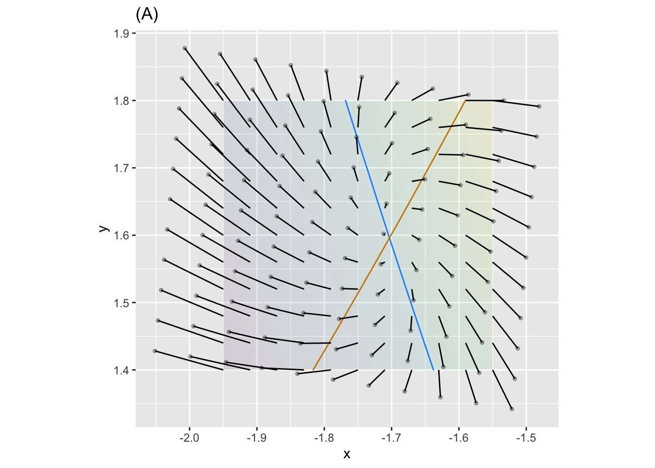
**Part A**  Is the fixed point in (A) stable or not?

Stable Unstable

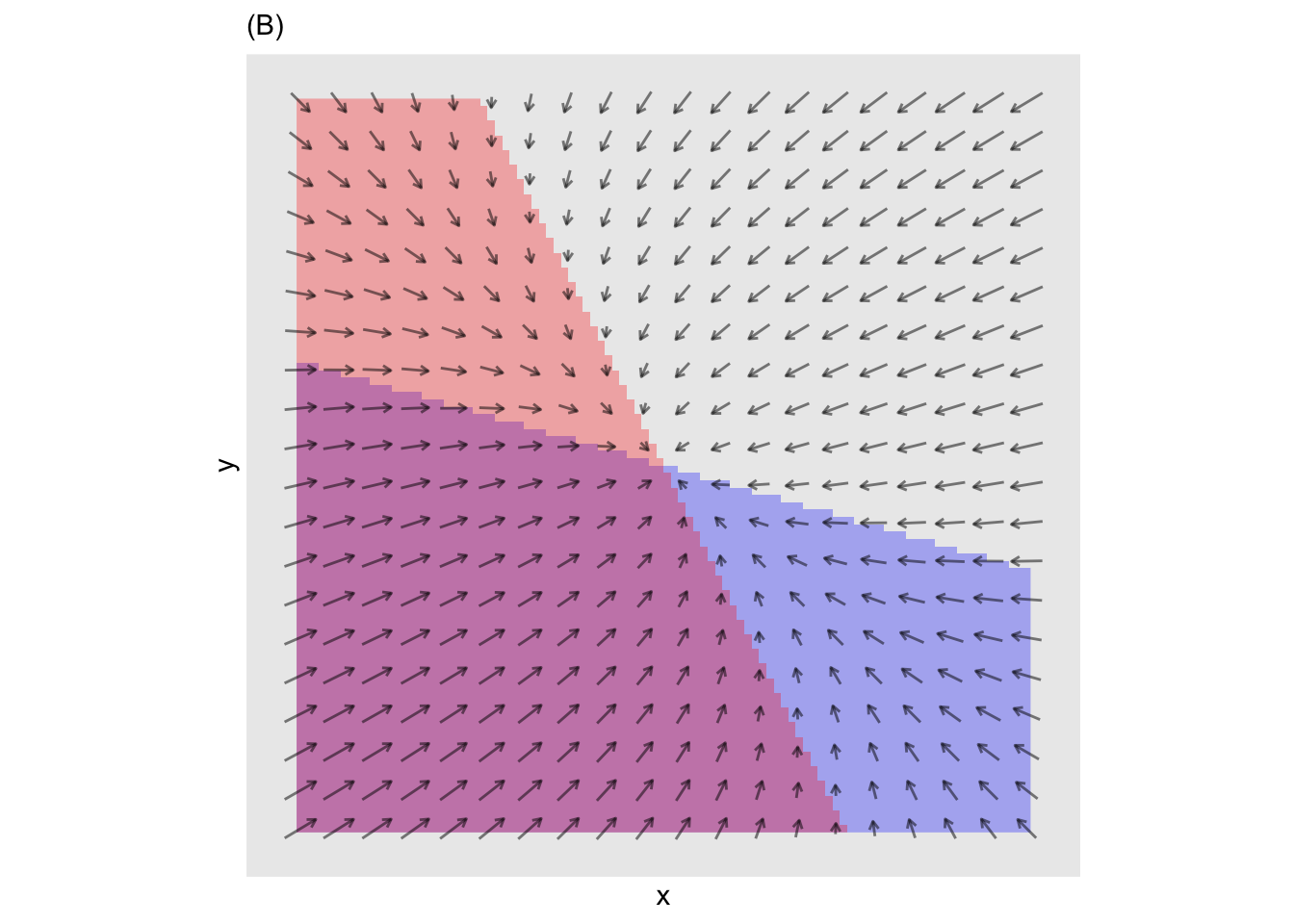
**Part B**  Is the fixed point in (B) stable or not?

Stable Unstable

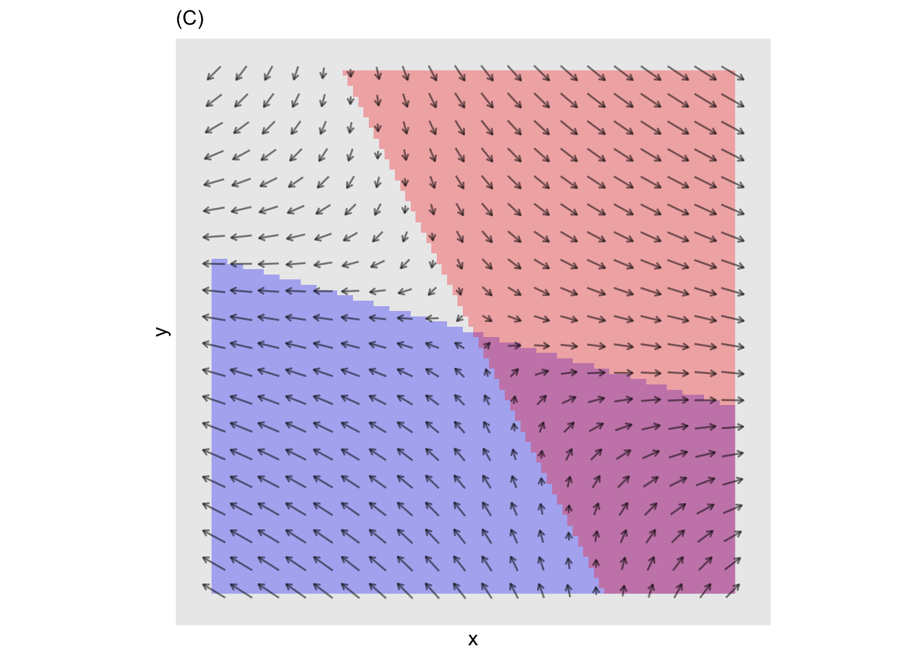
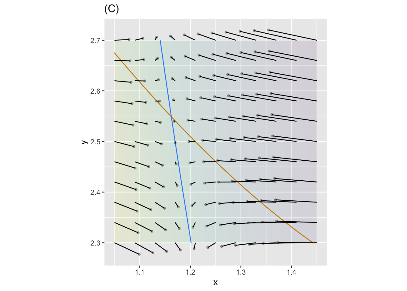
**Part C**  The fixed point in (C) is called a "saddle." It is stable in one direction and unstable in another. Which of these is correct?

Stable in y-direction and unstable in the x-direction
Stable in the x-direction and unstble in y

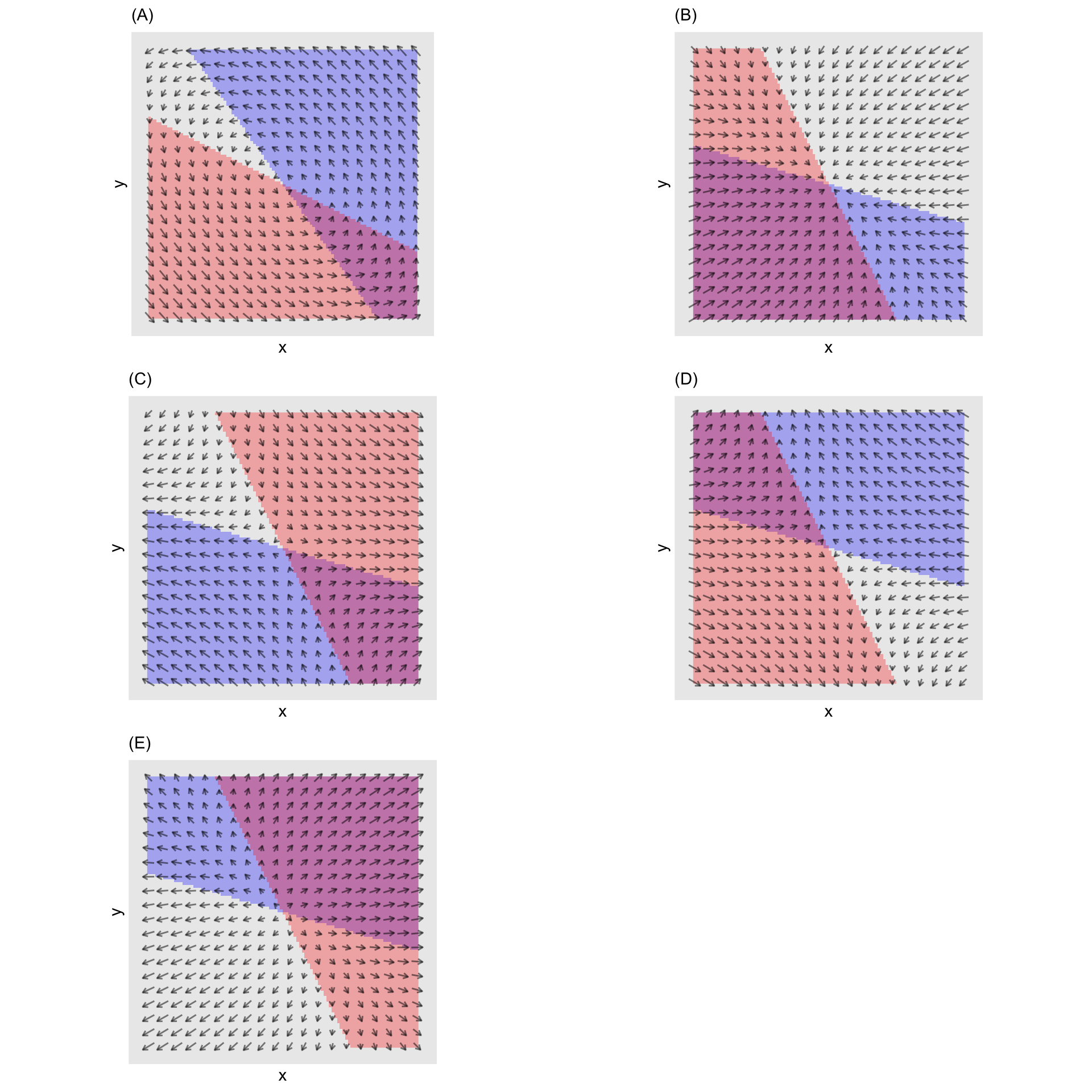
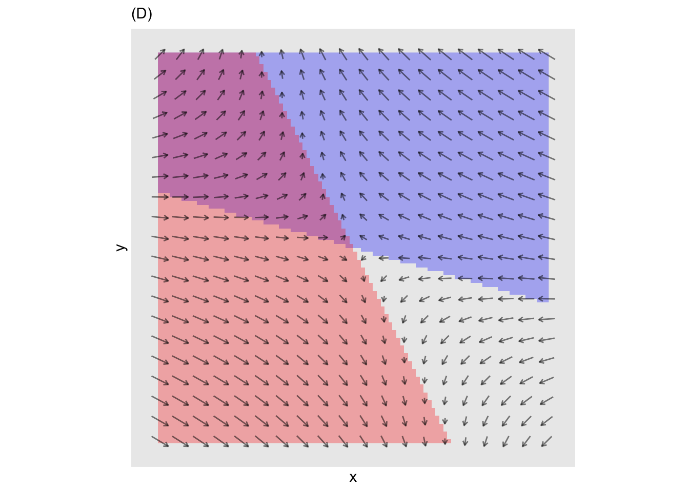
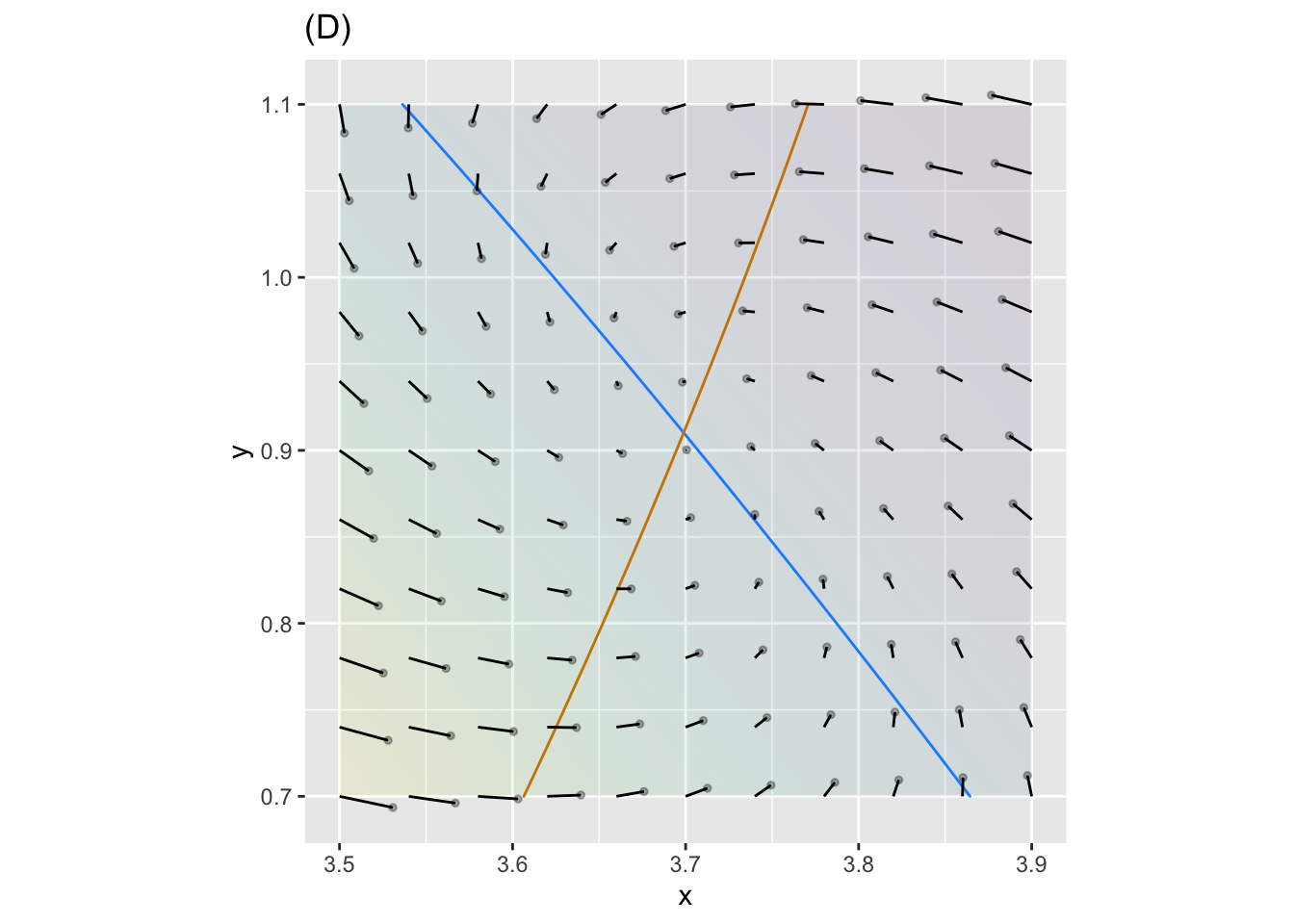
Here’s a system which has 4 fixed points in the region shown.

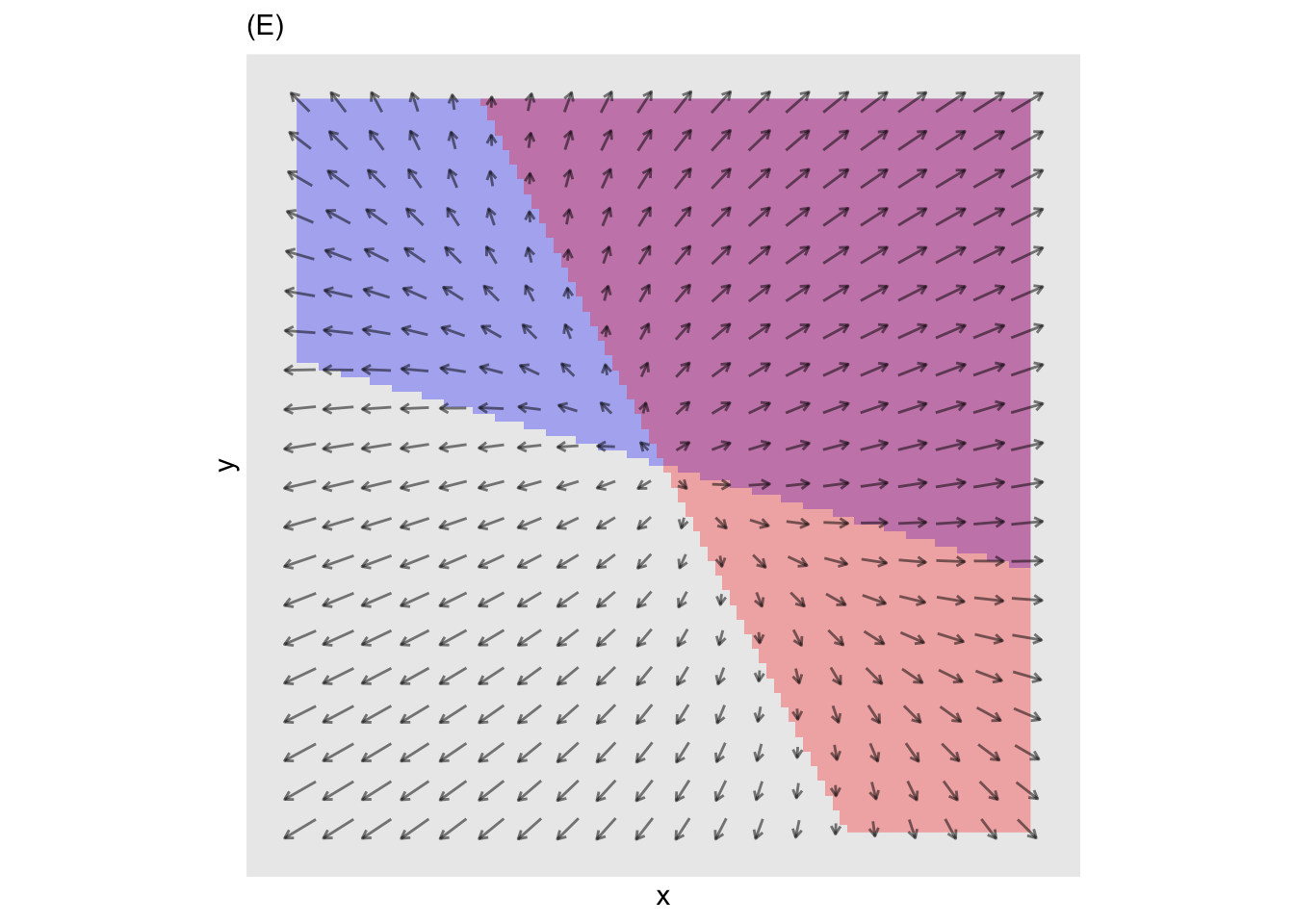
Plots (D) and (E) zoom in on two regions.

**Part D**  Which of the following is the best description of the behavior near the fixed point in (D)?

Stable and rotating clockwise
Stable and rotating counter-clockwise
Unstable and rotating clockwise
Unstable and rotating counter-clockwise

**Part E**  Which of the following is the best description of the behavior near the upper left fixed point in (E)? (Neutal stability means neither stable nor unstable; the trajectory just orbits around the fixed point.)

Unstable and rotating clockwise
Stable and rotating counter-clockwise
“Neutral stability” and rotating clockwise
“Neutral stability” and rotating counter-clockwise

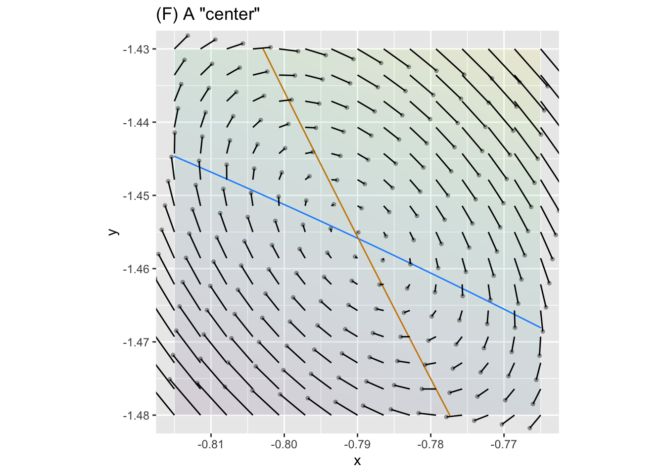
Let’s look a little more closely at the upper-left fixed point in graph (E):

The pattern in figure (F) is clockwise rotation around the fixed point. This kind of pattern is of fundamental importance in physics and engineering.

Exercise 3

**Part F**  In plot (A), how many fixed points are visible?

0 1 2 3 4 5

**Part G**  In plot (B), how many fixed points are visible?

0 1 2 3 4 5

**Part H**  In plot (C), how many fixed points are visible?

0 1 2 3 4 5

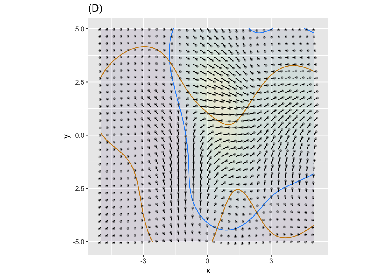
**Part I**  In plot (D), how many fixed points are visible?

0 1 2 3 4 5

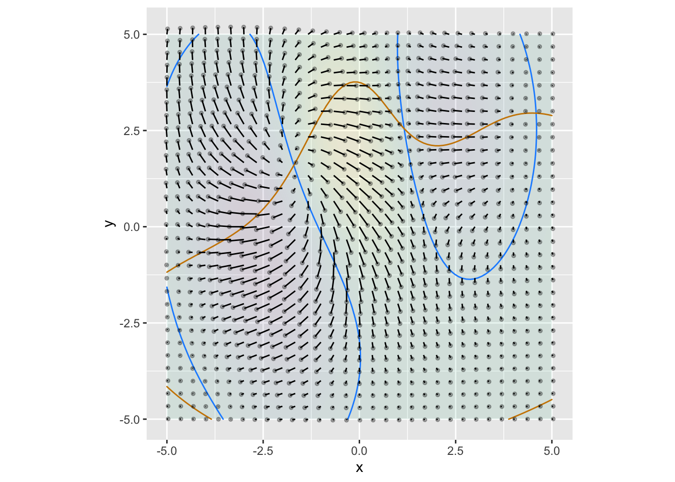
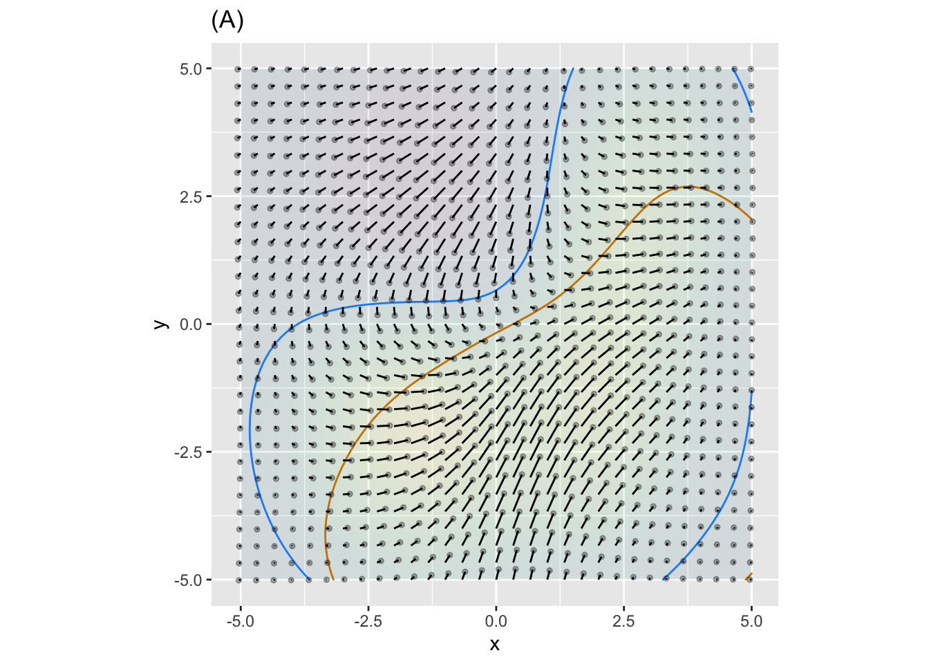
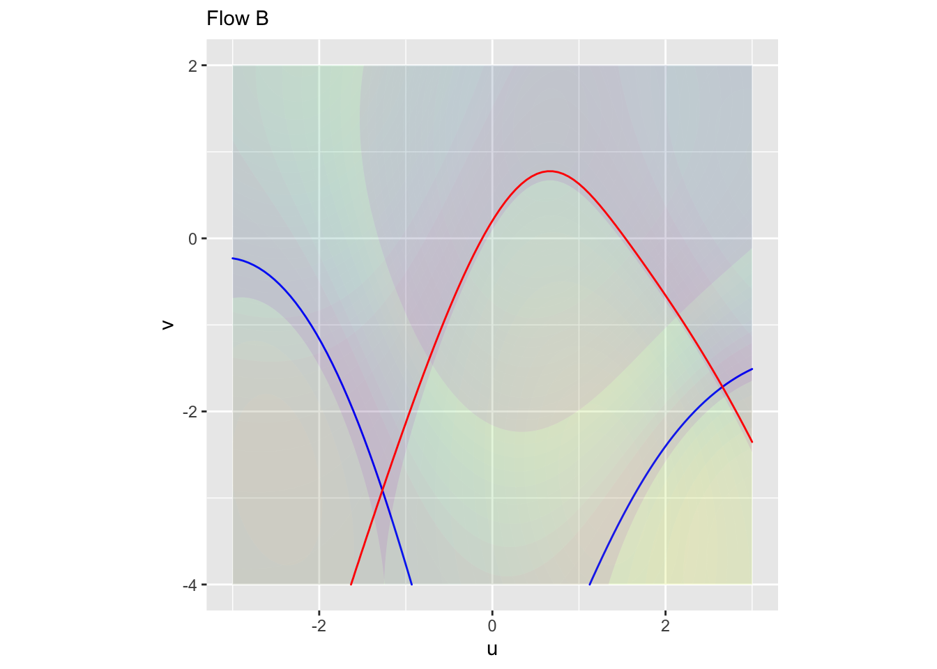
Exercise 4 In each of the following graphs, a flow field is annotated with a red contour and a blue contour. Your task is to determine whether a contour corresponds to a zero of the horizontal component of flow, a zero of the vertical component of flow, or neither. (Remember, if the contour is at a zero of the horizontal flow, the flow on the contour will be entirely vertical. And vice versa.)

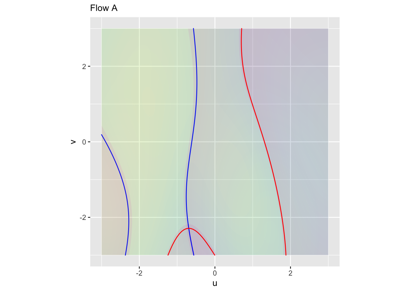
Plot A \(\color{blue}{\text{blue contour}}\):
1. Zero of horizontal flow
2. Zero of vertical flow
3. Neither
Plot A \(\color{red}{\text{red contour}}\):
1. Zero of horizontal flow
2. Zero of vertical flow
3. Neither

Plot B \(\color{blue}{\text{blue contour}}\):
1. Zero of horizontal flow
2. Zero of vertical flow
3. Neither
Plot B \(\color{red}{\text{red contour}}\):
1. Zero of horizontal flow
2. Zero of vertical flow
3. Neither

Exercise 5 The rabbit-fox system is nonlinear: \[\partial_t r = \alpha r - \beta r f\\ \partial_t f = - \delta f + \gamma rf\]

Write down, in English, the names of the Greek letters in the above formula.
Using algebra, find the fixed point \((r^\star, f^\star)\) of the rabbit-fox system.

Linearize the rabbit-fox system around the fixed point and write down the linearized dynamics in this form:

\[\partial_t r = A [r - r^\star] + B [f - f^\star]\\ \partial_t f = C [r - r^\star] + D[f - f^\star]\] Your should give the values of \(A, B, C, D\) in terms of the Greek letters of the nonlinear system.

\[\partial_t r = \left(\alpha + \frac{\beta\gamma}{\delta}\right) [r - r^\star] + \alpha [f - f^\star]\\ \partial_t f = - \delta [r - r^\star] + \left(\delta + \frac{\alpha\beta}{\delta}\right) [f - f^\star]\]

Exercise 6 ?fig-linearized-pendulum shows a flow field of the pendulum system and three pairs of trajectories, one pair for each of three initial conditions. Each trajectory starts at \(t=0\) and ends at \(t=6\).

A. Read the three different initial conditions from the graph.

B. The dark gray trajectories are for the original (nonlinear) pendulum system while the \(\color{magenta}{\text{magenta}}\) trajectories are for the linearized dynamics. Describe in words the differences in the trajectories for the nonlinear and the linearized dynamics.

C. The flow field corresponds to either the nonlinear (gray) or linearized (\(\color{magenta}{\text{magenta}}\)) dynamics. Which one is it?

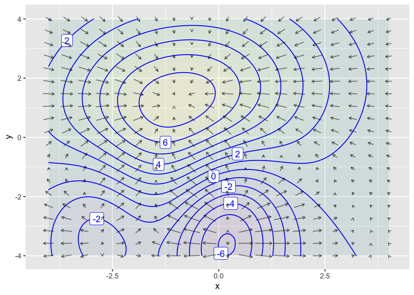
Exercise 7 In this exercise, you will work with a particular function f() of two variables. Construct the function this way:

f <- doodle_fun( ~ x + y, seed=103)

The goal of this exercise is to explore the connections between the optimization method of gradient ascent or descent and dynamical systems.

Here’s a plot of the function and its gradient field.

contour_plot(f(x, y) ~ x + y, domain(x=-4:4, y=-4:4)) %>%
  gradient_plot(f(x, y) ~ x + y, domain(x=-4:4, y=-4:4))

You can construct the \(x\) and \(y\) components of the gradient \(\partial_x f(x,y)\) and \(\partial_y f(x,y)\) of f() this way:

dx_f <- D(f(x, y) ~ x)
dy_f <- D(f(x, y) ~ y)

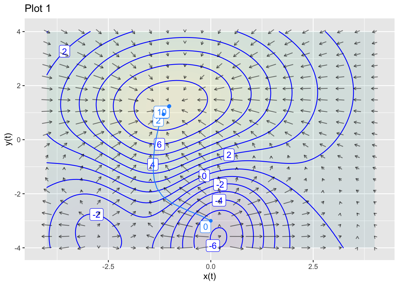
Use these two functions to define a dynamical system: \[ \partial_t x = \partial_x f(x,y)\\ \partial_t y = \partial_y f(x,y)\]

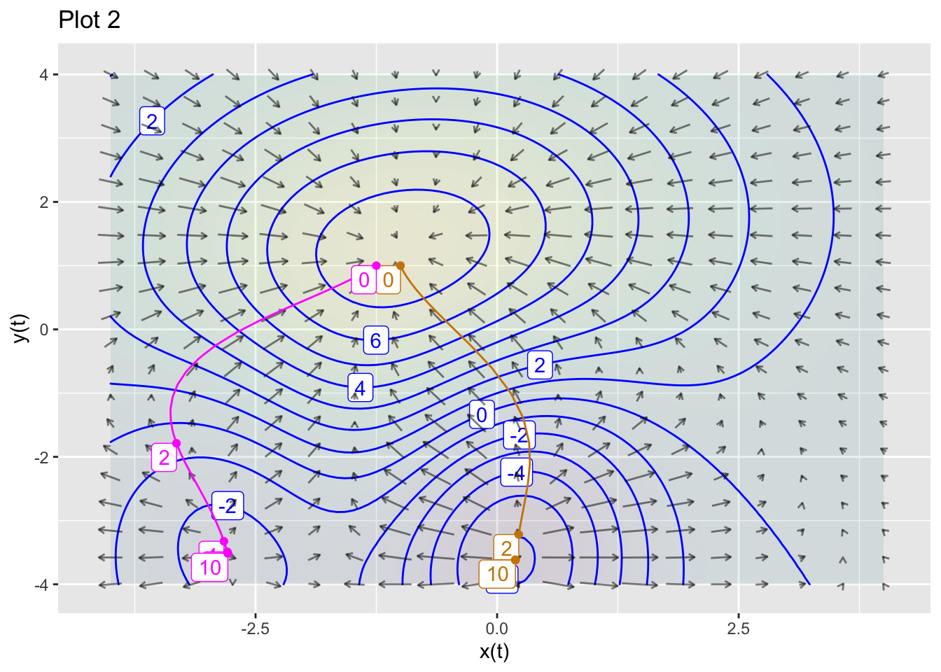
Use integrateODE() to integrate the equations numerically from the initial condition \((x=0, y=-3)\). Plot the resulting trajectory as a layer on top of the contour plot and gradient field. Make the time bounds in integrateODE() large enough to get very close to the high-point in the contour plot.
Modify the differential equations so that they correspond to gradient descent rather than ascent. Using the initial condition \((x=-1, y=1)\), numerically integrate the differential equations and, as in (1), plot the trajectory as a layer on the contour-plot/gradient-field. Make the time bounds large enough to get very close to a local minimum of \(f()\).
From (2), change the initial condition to \((x=-1.25, y=1)\) and plot the trajectory. What’s different from the result in (2).

Solution containing functions x(t), y(t).
Solution containing functions x(t), y(t).
Solution containing functions x(t), y(t).

No answers yet collected