Chap 9 Exercises
\[ \newcommand{\dnorm}{\text{dnorm}} \newcommand{\pnorm}{\text{pnorm}} \newcommand{\recip}{\text{recip}} \]
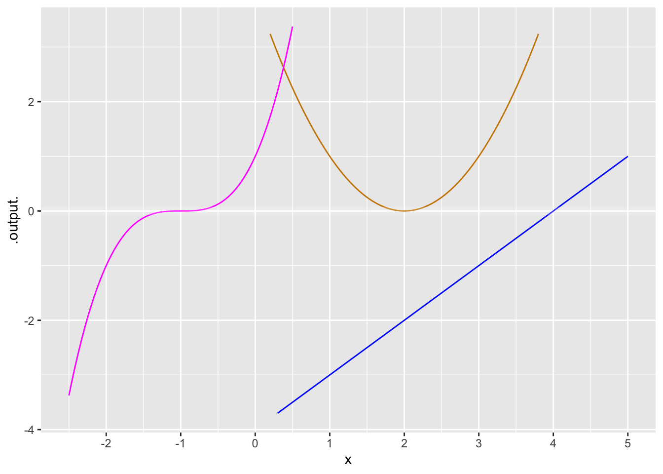
Exercise 1 Each of the three functions graphed below is a simple power-law function that can be written \(\left[\strut x-x_0\right]^n\). The three functions in Figure 1 have different values for \(x_0\) and for \(n\).
1a. For the \(\color{blue}{\text{blue}}\) function, what is \(x_0\)?
question id: local-shift-1a
1b. For the \(\color{blue}{\text{blue}}\) function, what is the order of the polynomial?
question id: local-shift-1b
2a. For the \(\color{orange}{\text{orange}}\) function, what is \(x_0\)?
question id: local-shift-2a
2b. For the \(\color{orange}{\text{orange}}\) function, what is the order of the polynomial?
question id: local-shift-2b
3a. For the \(\color{magenta}{\text{magenta}}\) function, what is \(x_0\)?
question id: local-shift-3a
3b. For the \(\color{magenta}{\text{magenta}}\) function, what is the order of the polynomial?
question id: local-shift-3b
Exercise 2 For each of the following, say whether the function \(f_?()\) is a linear combination, a multiplication, or a composition of the two simpler functions.
- \(f_a(t) \equiv \sin(e^x)\)
question id: dog-hunt-fabric-a
Use Active R chunk 1 to plot \(f_a()\) over the domain \(0 \leq t \leq 10\) and explain the obvious ways in which \(f_a()\) differs from the pattern-book \(\sin()\).
- \(f_b(t) \equiv e^x \sin(x)\)
question id: dog-hunt-fabric-b
Use Active R chunk 1 to plot \(f_b()\) over the domain \(0 \leq t \leq 10\) and explain the obvious ways in which \(f_b()\) differs from the pattern-book \(e^x\).
- \(f_c(t) \equiv e^{\sin(t)}\)
question id: dog-hunt-fabric-c
Use Active R chunk 1 to plot \(f_c()\) over the domain \(0 \leq t \leq 20\) and explain the obvious ways in which \(f_c()\) differs from the pattern-book \(e^x\).
Exercise 3 The function bigger() is defined piecewise in terms of two extremely simple functions. Each of the two simple functions has a contour plot with contours that are parallel. The piecewise combination of the simple functions has a more complicated contour plot, with each simple function’s parallel contours showing up in half of the domain. We will call these “pieces” of the domain.
Which of the following best describes the two pieces of the domain?
One is above and to the left of the line of identity (that is, \(y=x\)) and the other is below and to the right of that line.
One is \(x > 0\) and the other \(x \leq 0\)
One is \(x > 0\) and the other \(y \leq 0\)
question id: bigger-two
Exercise 4 The Heaviside function has two asymptotes.
Are they horizontal or vertical asymptotes?
question id: beech-ride-table-1
- What are the values reached assymptotically?
question id: beech-ride-table-2
Exercise 5
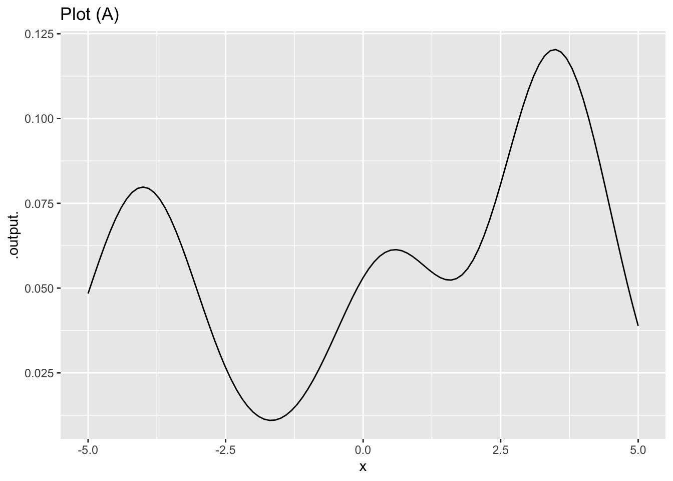
Figure 2 shows a function that is a linear combination of three x-shifted gaussian functions \[a_1 \dnorm(x-3.5) + a_2 \dnorm(x-0.5) + a_3 \dnorm(x-(-4))\]
Estimate the coefficients \(a_1, a_2\), and \(a_3\) for the function drawn in Plot (A). (Be sure to get the order right!)
\(a_1 = 0.3, a_2 = 0.15, a_3=0.2\)
\(a_1 = 0.15, a_2 = 0.2, a_3=0.3\)
\(a_1 = 0.2, a_2 = 0.3, a_3=0.15\)
\(a_1 = 0.15, a_2 = 0.3, a_3=0.2\)
question id: b-road-1-1
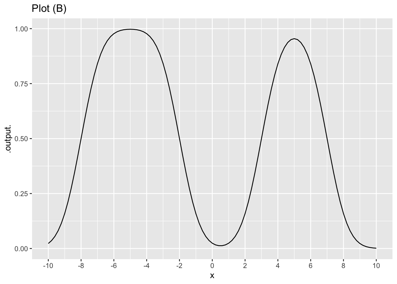
In Figure 3 each of the coefficients in the linear combination is either 1 or \(-1\). Recall that a handy fiducial point for the sigmoid function is the input at which the output is 1/2.
- Where are the fiducial points for the four sigmoids in Figure 3?
\(-8, -2, 3, 7\)
\(-6, -4, 0, 6\)
\(-9, -8, 1, 5\)
\(-2, 2, 4, 6\)
question id: b-road-1-3
- What are the coefficients on the respective sigmoids, in order from the leftmost to rightmost?
question id: b-road-1-4
Exercise 6 The Bargain Basement store wants to sell its goods quickly. Consequently, they reduce each product’s price \(P\) by 5% per day.
- If a jacket costs $80 today, how much will it cost in \(t\) days?
\(P = 80 - 5t\)
\(P = 80 - 4t\)
\(P = 80 - 0.05t\)
\(P = 80 (0.05)^t\)
\(P = 80 (0.95)^t\)
question id: chicken-choose-vase-1
Use Active R chunk 2 in answering the next question. Remember, to raise a number to a power, you can use an expression like 0.95^7.
- You decided that you like the $80 jacket, but you have a budget of only $60. How long should you wait before coming back to the Bargain Basement store?
question id: chicken-choose-vase-2
- The answer to question (1) is an exponential function, even if at first it doesn’t look like it. Which of these is the same function but written in the standard \(e^{kt}\) format?
\(80 \exp( \ln(0.95) t)\)
\(0.95 \exp(80 t)\)
\(80 \exp(-\ln(0.95) t)\)
\(0.95 \exp(\ln(80) t)\)
question id: chicken-choose-vase-3
Exercise 7 If you are unlucky and develop a serious ear or throat or other infection, and if the infection is bacterial and not viral, you may be prescribed antibiotics. You probably know how it goes. You go to the pharmacy to pick up a bottle of pills. There might be anywhere between 10 pills and 40. The directions will certainly tell you to make sure to finish the bottle; to take the full course of medication. It may say take a pill twice a day, or three times, or every six hours, perhaps with food.
The details of this regimen are determined largely by the details of whether food inhibits or buffers absorption of the medicine and by the efficiency by which your body metabolizes the medicine and then removes it from your blood via your liver.
Modeling this process—often called the pharmacokinetics of the drug—is an important step in drug development. A simple but effective model of the drug concentration over time is a piecewise function: zero before you take the pill, then an exponential decay from an initial level of one unit after you take the pill.
The shape of the pill() function is seen in Figure 4. Another part of the model is the therapeutic threshold, the minimal concentration for medical effectiveness. Keep in mind that this is a model. In reality, the drug not is absorbed instantaneously as in the model, and the medical effectiveness varies smoothly with concentration rather than being an all-or-nothing affair.
Warning: All aesthetics have length 1, but the data has 101 rows.
ℹ Please consider using `annotate()` or provide this layer with data containing
  a single row.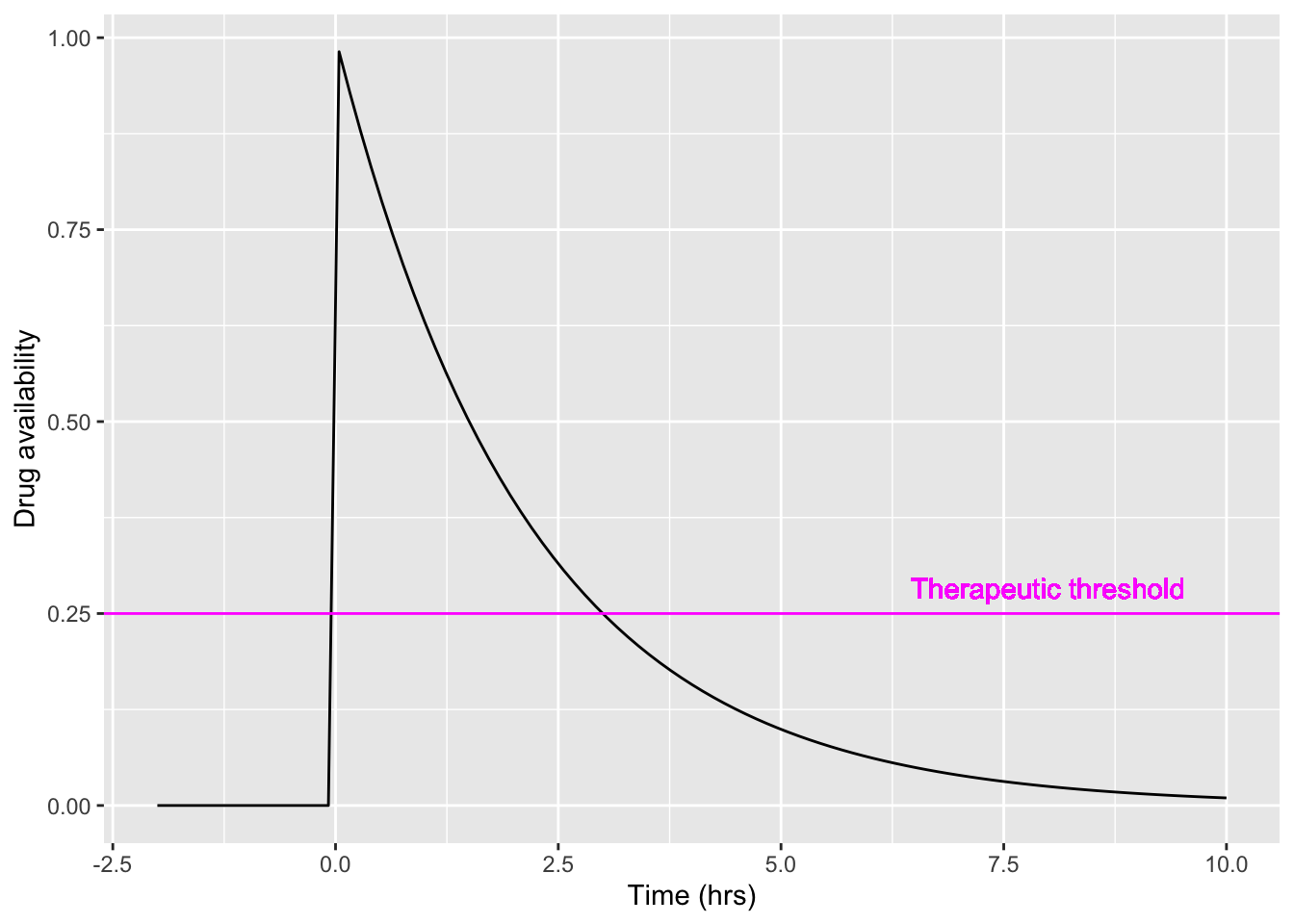
gf_text() function adds a label to the plot. You aren’t expected to master label making.)
The critical features of the model are the half-life of the drug in the body and the therapeutic threshold, both of which depend on the particular drug in question.
- What is the half life of the drug depicted in the Figure 4?
question id: goat-walk-window-1
Figure 4 shows the availability from a single pill. The goal of taking multiple pills, spread out over time, is to keep the drug availability above the therapeutic threshold for an extended time, e.g. 10 days. There are three parameters to the therapy: how often you take a pill, and the dose delivered by a single pill, and the medicine’s half-life.
- Occasionally, the prescription directs you to take a single pill once a day. Suppose the half-life of the medicine is 3 hours. How big would the dose
Aneed to be to keep the availability above a threshold of 0.25 for a 24-hour period?
question id: goat-walk-window-2
Let’s explore a familiar-sounding directive: Take one pill every six hours. We can model this by a linear combination of time-shifted pill() functions. Each pill provides a dose of size A. Active R chunk 4 shows the overall function for an entire day after the first dose.
The graph shows that the drug is above the therapeutic threshold (0.25) for the entire first day (0-24 hours).
- From the graph of drug availability versus time, do you think continuing the one-pill-every-6-hours regimen will continue to keep the drug level over the therapeutic threshold for the remainder of the course of treatment? Explain why or why not.
Let’s switch to an one-pill every 8 hour regimen, the pills being taken at midnight, 8am, and 4pm, …
- How big a dose
Awill be needed to keep the drug availability above the therapeutic threshold for the entire course of treatment? (Hint: Construct a function analogous tosix_hours()that simulates a pill every 8 hours. Plot out the drug availability over the 24 hours of the first day. Then vary the doseAuntil you find the minimum dose that keeps the availability over the threshold of 0.25 for the entire day.)
question id: goat-walk-window-4
- Suppose the instructions were to take 2 pills when you start treatment and then an additional pill every 8 hours. Active R chunk 5 creates and graphs the appropriate function.
How big a dose A would be needed to keep the drug availability above the therapeutic threshold for the entire course of treatment?
question id: goat-walk-window-5
- Which of the three regimens described (6-hour, 8-hour, 8-hour-double-first-dose) involves the smallest total dose for a drug regimen lasting 10 days? (The total dose is the sum of the doses for each pill administration.)
question id: goat-walk-window-6
Exercise 8
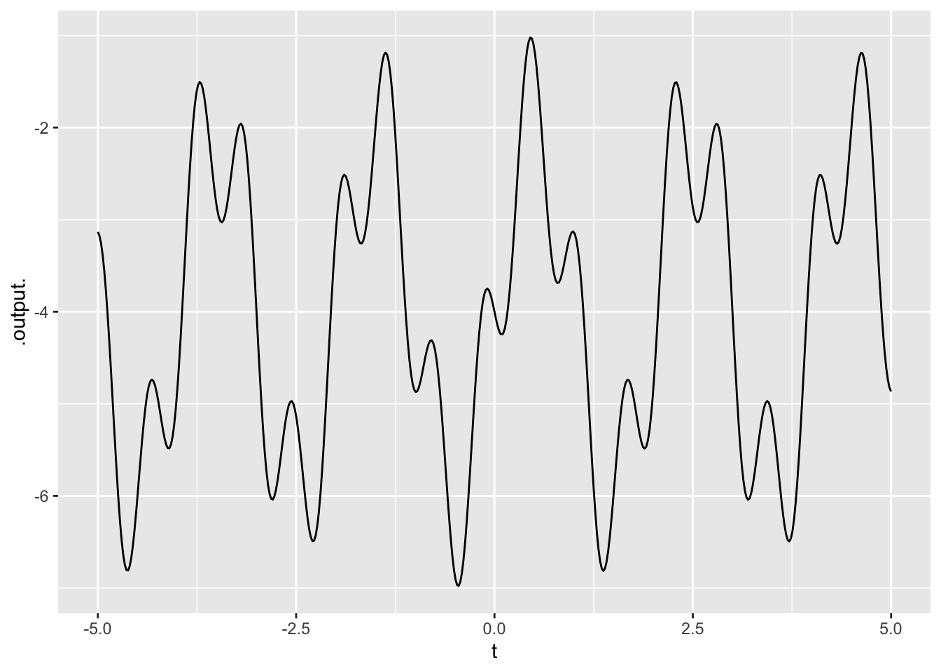
\[A_1 \sin\left(\frac{2\pi}{2}t\right) + A_2 \sin\left(\frac{2\pi}{0.6} (t-.3)\right) + A_3 \tag{1}\]
- What is \(A_3\)?
question id: two-sines-1a
- What is \(A_1\)?
question id: two-sines-1b
- What is \(A_2\)?
question id: two-sines-1c
Exercise 9 Figure 6 shows two gaussian functions \(g_1(t)\) and \(g_2(t)\) with different means and standard deviations.
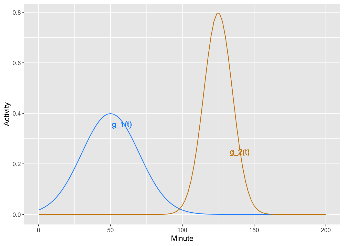
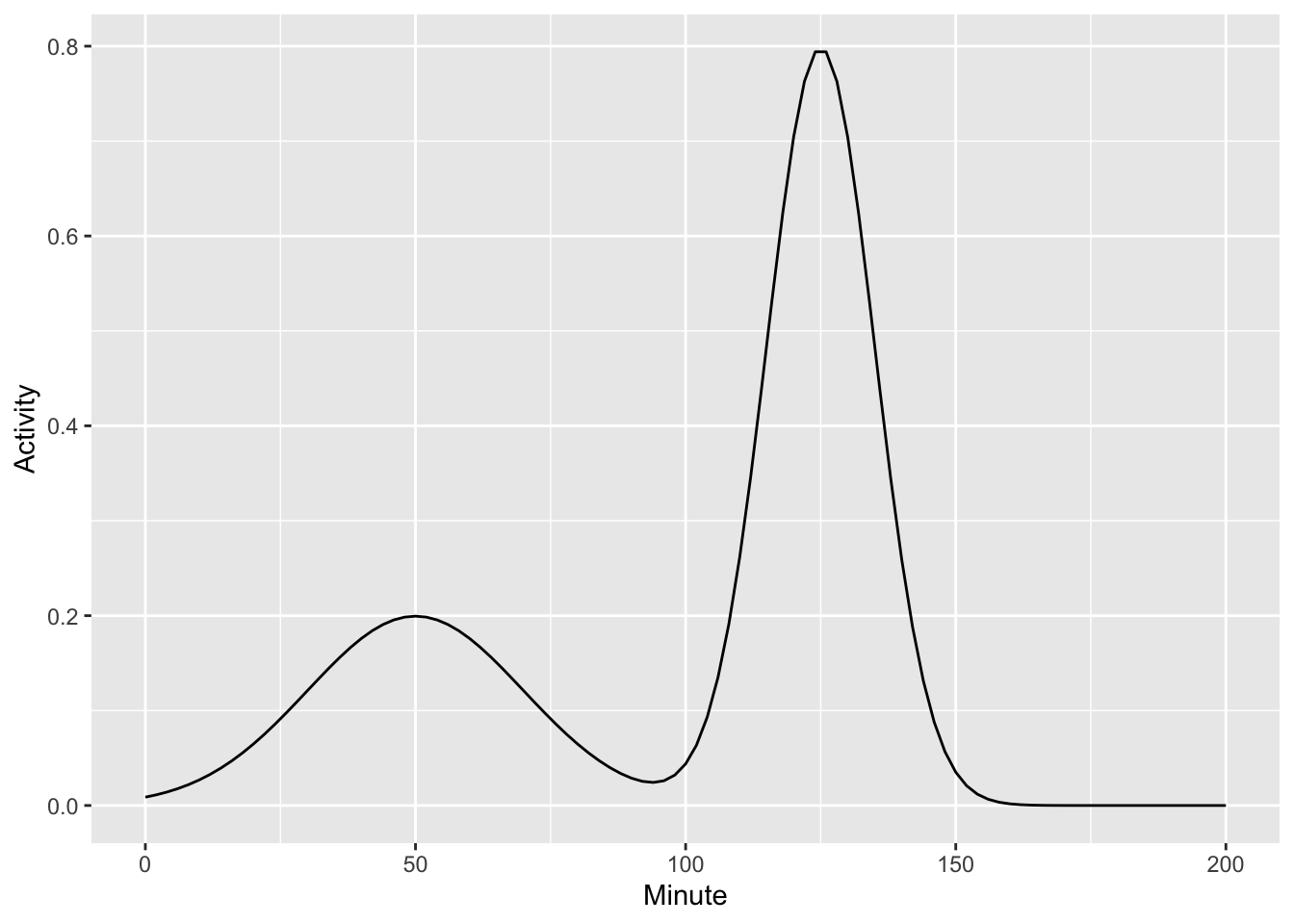
- What is the linear combination of \(g_1(t)\) and \(g_2(t)\) shown in Figure 7?
\(0.5\,g_1(t) + g_2(t)\)
\(g_1(t) + 0.25\,g_2(t)\)
\(g_1(t) + 2\,g_2(t)\)
question id: daily-digital-09-QA17

- Which linear combination of \(g_1(t)\) and \(g_2(t)\) is shown in Figure 8?
\(g_1(t) - 2\, g_2(t)\)
\(g_1(t) - g_2(t)\)
\(0.5\,g_1(t) - 0.5\, g_2(t)\)
\(-g_1(t) - g_2(t)\)
question id: daily-digital-09-QA18
Exercise 10
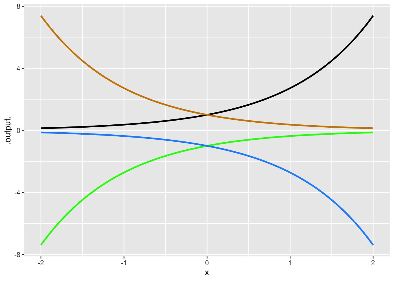
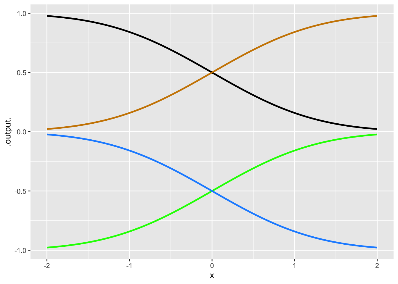
- One of the curves in Figure 9 is a pattern-book function. Which one?
question id: flipping-1-1a
- Taking \(f()\) to be the pattern-book function in Figure 9, which one of the curves is \(f(-x)\)?
question id: flipping-1-1b
- One of the curves in Figure 10 is a pattern-book function. Which one?
question id: flipping-1-2a
- Taking \(f()\) to be the pattern-book function in Figure 10, which one of the curves is \(-f(x)\)?
question id: flipping-1-2b
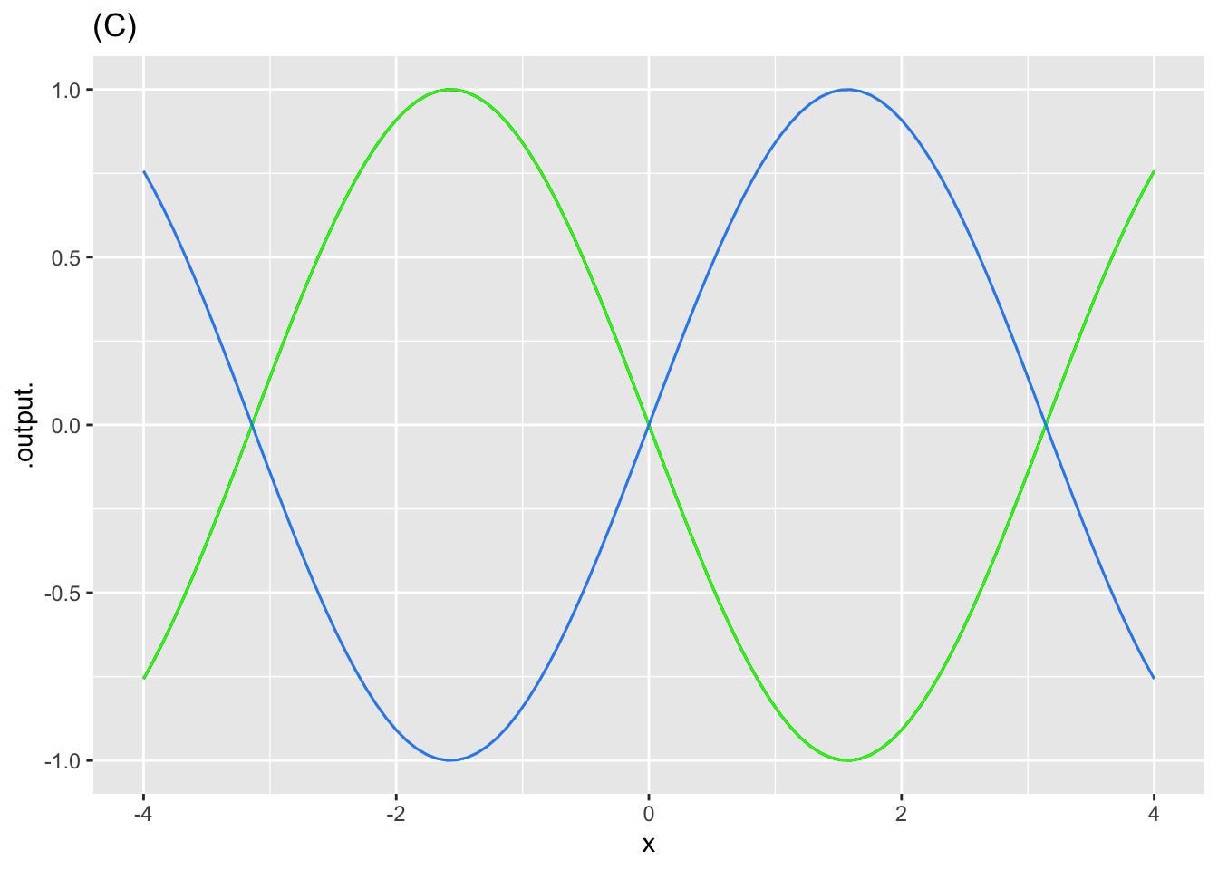
- The blue curve in Figure 11, as you know, is the sinusoid pattern-book function. Which of these functions is the green curve?
\(\sin(-x)\)
\(-\sin(x)\)
\(-\sin(-x)\)
Both \(\sin(-x)\) and \(-\sin(-x)\)
Both \(\sin(-x)\) and \(-\sin(x)\)
question id: flipping-1-3a
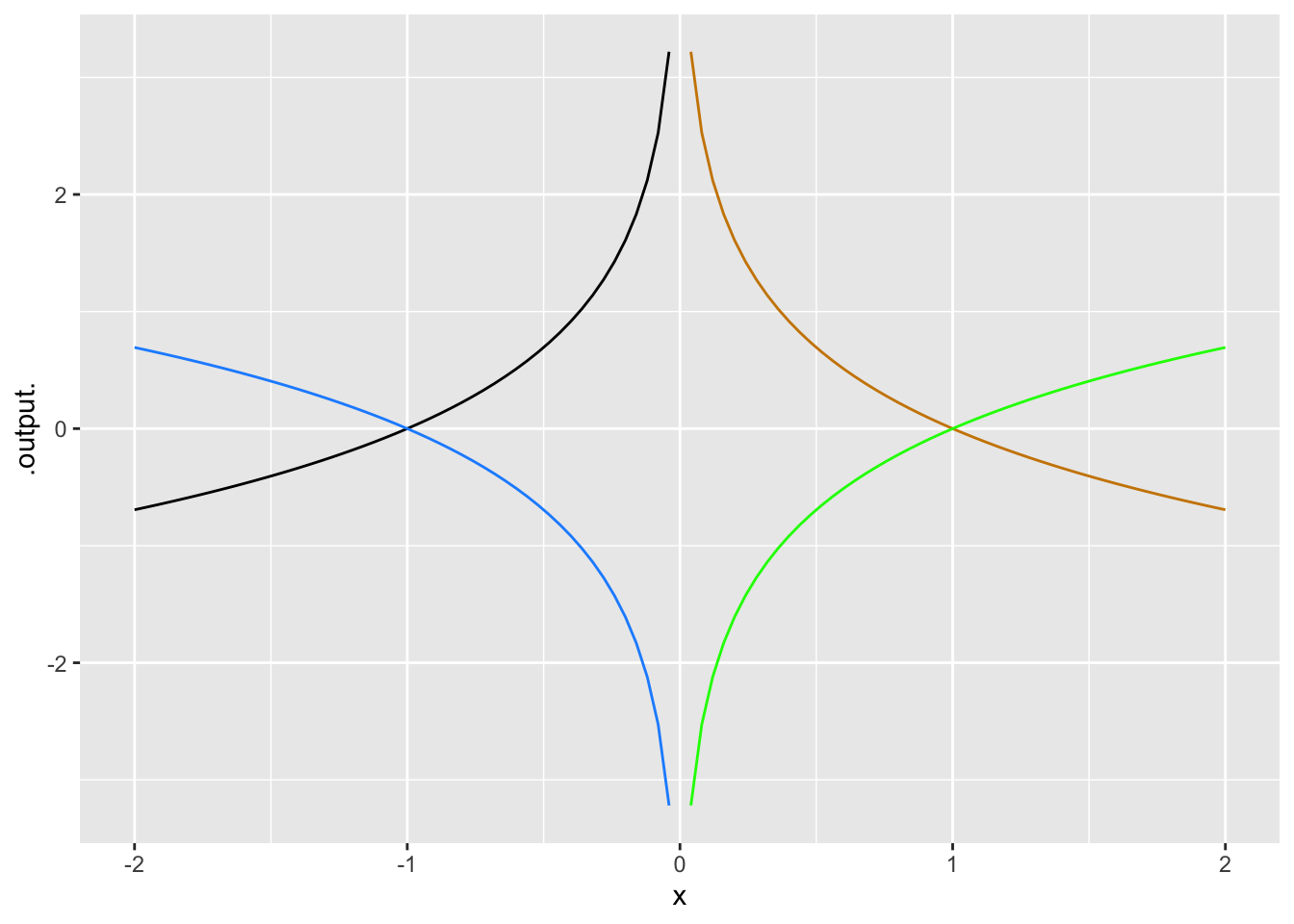
- One of the curves in Figure 12 is a pattern-book function. Which one?
question id: flipping-1-4a
- Taking \(f()\) to be the pattern-book function in Figure 12, which one of the curves is \(-f(-x)\)?
question id: flipping-1-4b
Exercise 11 Here is an interactive R chunk to use in answering the following questions:
- What is the shape of the graph of the composition \(\pnorm(\pnorm(x))\)?
question id: compose-1-1
- What is the shape of the graph of the composition \(\pnorm(\dnorm(x))\)?
question id: compose-1-2
- What is the shape of the graph of the composition \(\dnorm(\pnorm(x))\)?
question id: compose-1-3
- What is the shape of the graph of the composition \(\ln(\dnorm(x))\)?
question id: compose-1-4
- What is the shape of the graph of the composition \(\ln(x^2)\)?
question id: compose-1-5
- What is the shape of \(\exp(x^2)\)?
question id: compose-1-6
- What is the shape of \(\exp(-x^2))\)?
question id: compose-1-7
- What is the range of \(\sin(1/x)\)?
\(-1 \leq \sin(1/x) \leq 1\)
\(\infty < \sin(1/x) < \infty\)
\(0 \leq \sin(1/x) < \infty\)
\(-\infty < \sin(1/x) \leq 1\)
question id: compose-1-8
- What is the range of \(1/\sin(x)\)?
\(-1 \leq | \sin(1/x) |\)
\(\infty < \sin(1/x) < \infty\)
\(0 \leq \sin(1/x) < \infty\)
\(-\infty < \sin(1/x) \leq 1\)
question id: compose-1-9
- What is the shape of the graph of the composition \(\ln(\pnorm(x))\)?
a rise followed by an horizontal asymptotic approach to 0 as \(x\rightarrow \infty\)
a fishhook
a parabola
question id: compose-1-10
Exercise 12 Figure 13 shows how the intensity of light from the sun depends on distance \(r\). Wikipedia link The intensity is the number of photons per unit area. Imagining each red line to be the path followed by one photon, the intensity can be calculated by the area of the surfaces at distance \(r\), \(2r\), and \(3r\).
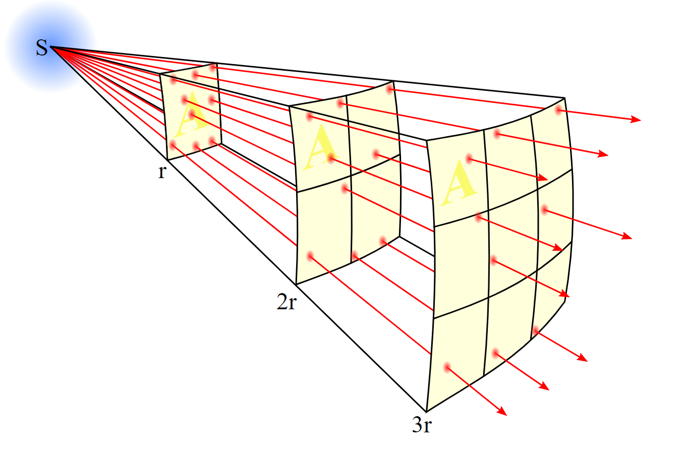
Which of these functional forms best models intensity \(\cal I\) as a function of distance \(r\)?
Proportional: \(\cal I(r)\equiv ar+b\)
Power-law: \(\cal I(r)\equiv Ar^p\)
Exponential \(\cal I(r)\equiv Ae^{kr}+C\)
Sine: \(\cal I(r)\equiv A\sin \left(\frac{2\pi}{p}(r-r_0)\right)+B\)
Sigmoid \(\cal I(r)\equiv A\cdot \pnorm(r,mean,sd)+B\)
Gaussian \(\cal I(r)\equiv A\cdot \dnorm(r,mean,sd)+B\)
question id: dolphin-burn-clock-1
Exercise 13 According to data from the US National Health and Nutrition Evaluation Survey, the average height of adult females is 157 cm vs 167 for adult males. The standard deviations are 17 cm and 22 cm respectively. A good model for the person-to-person variation for females is dnorm(height, mean = 157, sd = 17) and similarly for males.
To see the overall distribution of adult height, regardless of sex, make a linear combination of the distribution for females and for males, giving each a scalar of one-half (since the population is roughly 50-50 female/male).
In Active R chunk 6, construct the linear combination function for the overall distribution. Use the scaffolding to plot out the distributions for the individual sexes and the overall distribution.
Some people erroneously think that since the mean height of men is larger than women by 10cm, you can readily distinguish between the sexes based on height. However, notice that the overall distribution (plotted in black) does not show a dip between the sexes: there is no clear separation based on height.
As a thought experiment, let’s increase the separation in mean height from the actual value of \(167-157=10\) cm to something larger. You can increase the separation by 5 cm, for example, by making the men’s mean height 167+5.
What’s the smallest increase in separation (in cm) that produces a barely visible dip between the sexes in the overall height distribution?
question id: tg4
Exercise 14 The data points in Active R chunk 7 were collected by astronomer Tycho Brahe (1546-1601) and used by Johannes Kepler (1571-1630) to develop his theory of the motion of planets. The data record the estimated distance from Mars to the Sun as a function of time. They are not a continuous record because Mars can’t be observed when it is on the other side of the Sun from Earth.
The function that Kepler wanted to fit to the data is
\[dist(t) \equiv A \sin\left(2\pi (t - t_0 \right)/P + B \tag{2}\]
Math expression 2 has two coefficients, \(A\) and \(B\), as well as two nonlinear parameters \(P\) and \(t_0\).
The code in Active R chunk 7 plots Kepler’s data along with a very poorly fitting model.
Ignore for the moment the nonlinear parameters, that is, the period and time shift of the sinusoid.
Good values for the linear coefficients \(A\) and \(B\) can be estimated by eye. Modify the \(A\) and \(B\) parameters to produce a sinusoid that nicely covers the range of the data.
I confirm honorably that I have found nice \(A\) and \(B\) parameters.
I haven’t had the chance yet to complete this task.
question id: kepler-linear
Nonlinear parameters are much harder to find. Try to figure out values for \(P\) and \(t_0\) that bring the model function into close alignment with the data. Hint: The collected data cover every orbit of Mars during the time span in the graphical domain, so a good first guess is to look at the time difference between successive clusters of data points.
I confirm honorably that I have found pretty reasonable \(P\) and \(t_0\) parameters.
I haven’t had the chance yet to complete this task.
question id: kepler-nonlinear
Exercise 15 Epidemics are often modeled as a series of “waves.” Each wave involves different people. Let’s imagine two epidemic waves, one passing through the “blue” population and a smaller one through the “orange” population, like this:
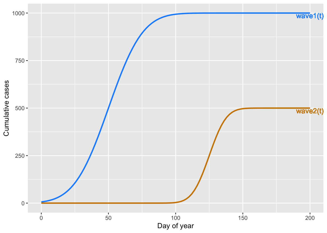
Assuming that the data collectors have no way to distinguish between red and blue cases, they would just be able to count the total number—red and blue—accumulated up to each day. That is, the epidemic would look like just one curve. Figure 15 shows four different candidates for this curve.
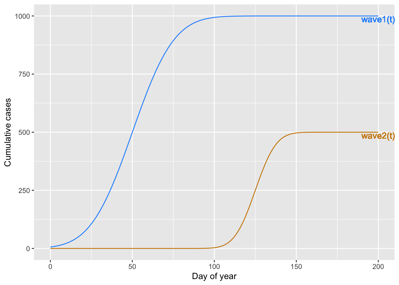
- Which of the following curves would the overall epidemic look like? (The colors are just to help you distinguish the different functions)
question id: daily-digitial-09-QA14
Each of the functions shown in Figure 15 is a “linear combination” of the brown function and the blue function in ?fig-arith-with-funs. The real total cumulative cases is “wave1(t)” plus “wave2(t)”. The other functions are made up and are irrelevant to the real epidemic. Still, we can ask what arithmetic combination of “wave1(t)” and “wave2(t)” was used to create the made-up function.
- For made-up function (A) in the graph, what was the linear combination?
1000 - wave1(t) + wave2(t)
2 wave1(t) - 3 wave2(t)
1000 + wave1(t) - wave2(t)
question id: daily-digital-09-QA16
Exercise 16 The graph shows (in black) a function constructed as the product of two basic modeling functions. The graph also shows a pair of blue curves that encompass the black function. These are called the envelope of the black function.
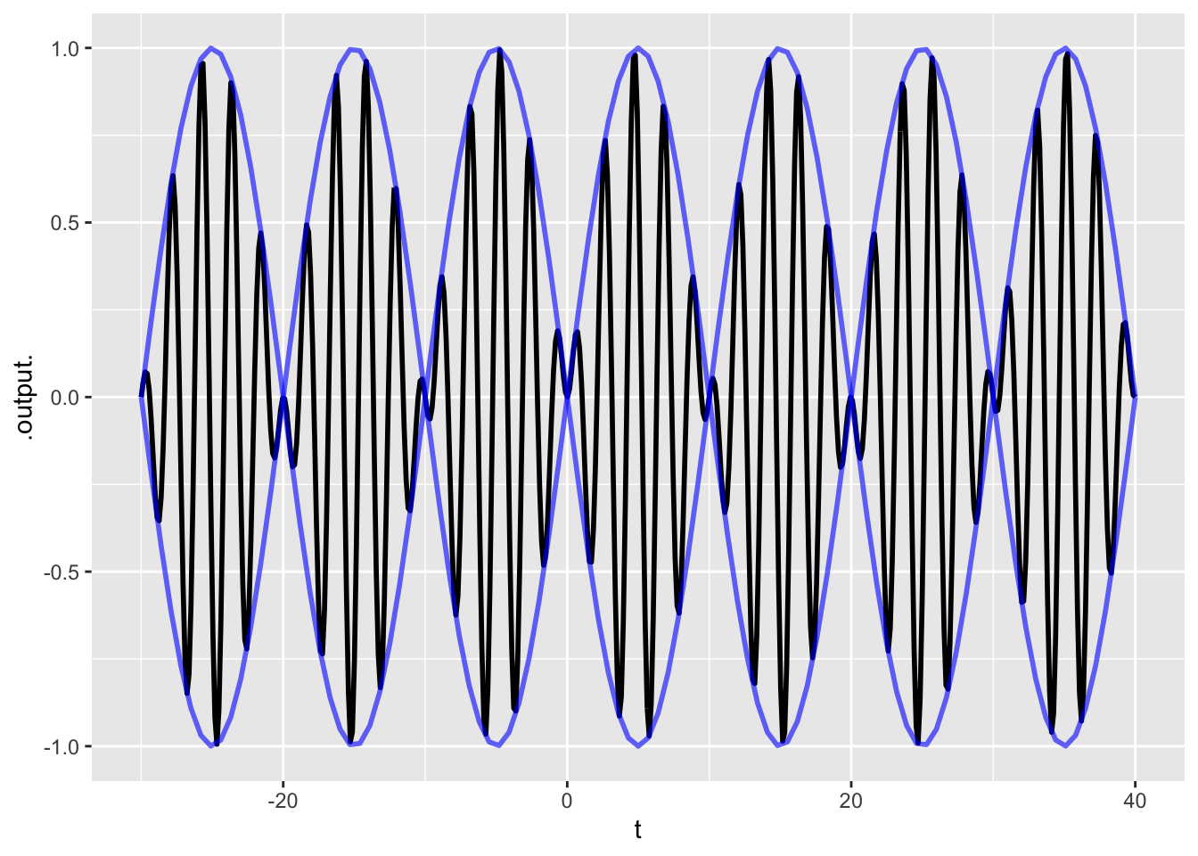
- What are the two basic modeling functions being multiplied?
A sinusoid and another sinusoid with a faster period.
A gaussian and a sinusoid.
A sigmoid function and a sinusoid.
question id: sin-in-sin-1
- What is the period of the envelope?
question id: sine-in-sine-2
Exercise 17 Here, in traditional mathematical notation, are the equations for calculating the length of daylight as a function of latitude and day number (1-365). First you calculate \(y()\), then the solar declination, then the hour-angle, then use the result to find the length of daylight.
\[y(\text{day}, \text{hour}) \equiv (2\pi/365) \times(\text{day} - 1 + (\text{hour}-12)/24)\]
\[\text{declination}(y) \equiv 0.006918-0.399912\,\cos(y)+0.070257\,\sin(y) -\\ 0.006758\,\cos(2*y)+0.000907\,\sin(2*y)-0.002697\,\cos(3*y)+0.00148\,\sin(3*y)\]
\[\text{hour\_angle}(L, \delta) \equiv \text{acos} \left(\strut\frac{\cos(90.833)}{\cos(L) \cos(\delta) - \tan(L)\tan(\delta)}\right)\] where \(\delta\) is the solar declination.
\[\text{daylight\_length}(\text{hour\_angle}) \equiv 2 \ \frac{\text{hour\_angle}(L, \delta)}{15}\]
Use Active R chunk 8 to implement these four functions in R. (The trig functions are spelled the same in R as in traditional notation.)
You will need to put these four functions together for the final calculation of daylight length. Active R chunk 9 shows how.
How long is the day on April Fools Day (\(n=90\)) at Latitude 39\(^\circ\)N? (Use
question id: april-fools
Exercise 18 It is very common in communications systems to have a signal that is a sine-wave carrier that is modulated by another function. That is, the carrier is multiplied by the other function: waveform(t) = modulator(t) \(\times\) carrier(t).
The interactive R chunks each have an examples in which a sine with a period of about 2 units is modulated by another function. In each case, that other function is one of the modeling functions we have studied.
- Of what sort is the function that is modulating the carrier?
question id: multiplying-functions-a
- Of what sort is the function that is modulating the carrier?
question id: multiplying-functions-b
- Of what sort is the function that is modulating the carrier?
question id: multiplying-functions-c
- Of what sort is the function that is modulating the carrier?
question id: multiplying-functions-d
Activities
Exercise 19
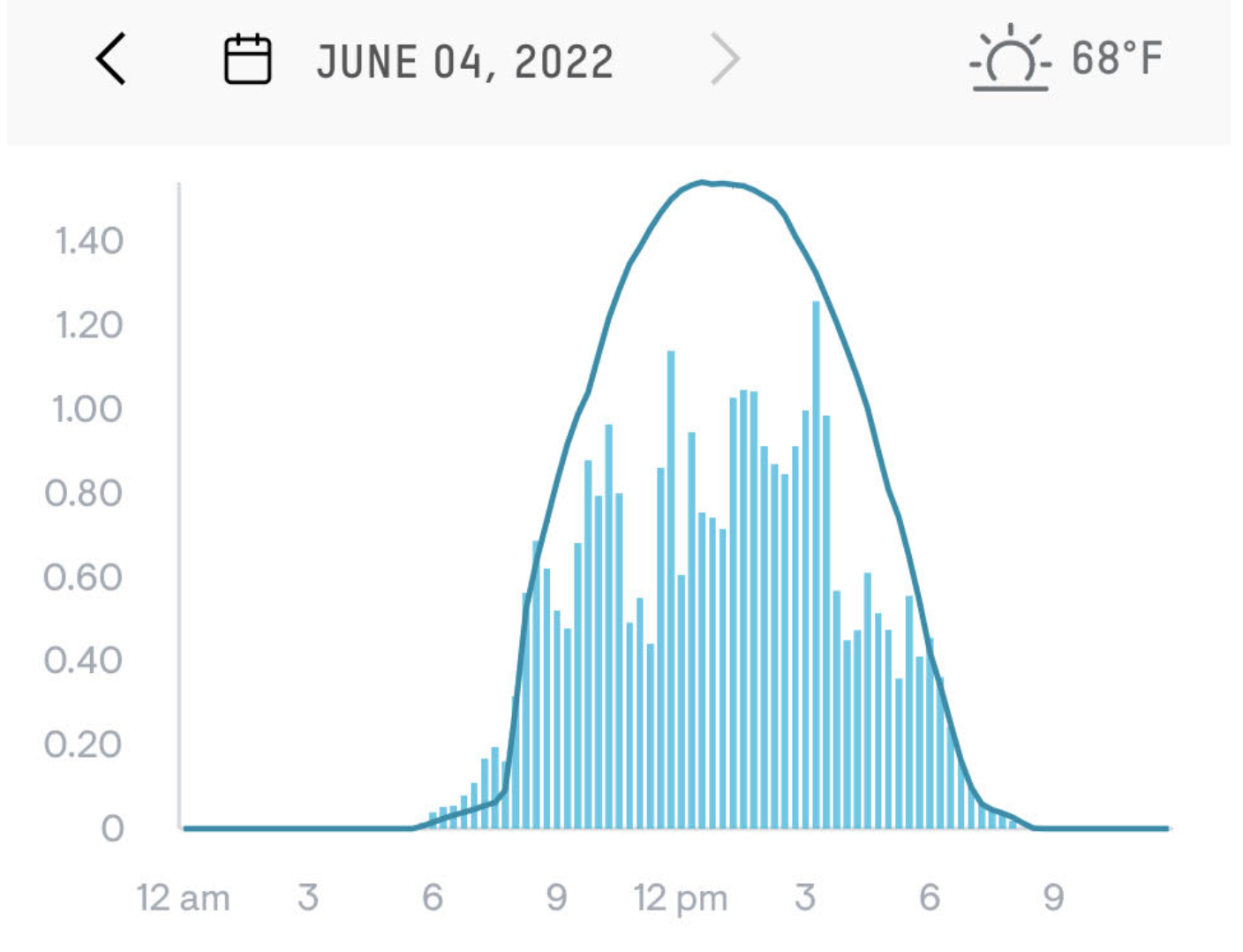
Figure 16 comes from the monitoring app for a photovoltaic (solar electricity) array on two consecutive days in June 2022. The vertical axis is in kilowatts (power). The overall pattern for June 4 is a bump function with a peak around 13:00 falling to zero at 6am and 9pm. (13:00 is roughly solar noon, due to daylight savings time.) We’ll call this function sun(t). June 3 shows a more complex pattern, due to passing clouds that diminish the available sunlight.
A reasonable model for the June 3 pattern is the bump function sun(t) multiplied by an irregular function of time representing the clouds. Let’s call it cloudiness(t), imagining that the range is from 0 (dark, obscuring clouds) to 1 (no clouds at all). The power produced is therefore
power(t) \(\equiv\) solar(t) \(\times\) cloudiness(t)
Refering to Figure 16, sketch out the graph of cloudiness(t) for June 3.