Chap 27 Exercises

\[ \newcommand{\dnorm}{\text{dnorm}} \newcommand{\pnorm}{\text{pnorm}} \newcommand{\recip}{\text{recip}} \]

Exercise 2 Here’s the Taylor polynomial expansion of $\sin(x)$ about a center $x_0$: \[p(x) = 1/2 - \frac{\sqrt{3}/{2}}{2!} (x - x_0)^2 + \frac{1/2}{4!} (x - x_0)^4 + \cdots\] Which of the following is the numerical value of $x_0$? (Hint: Remember that the coefficients involve the function and its derivatives evaluated at $x_0$ as described in [Faulty cross reference: high-order-approx].

Exercise 3 Consider the function $f(x) \equiv (x - 3)^2$.

Using ordinary algebra, $f(x)$ can be expanded as $(x^2 - 6 x -9)$. Consider \[p(x) = -9 - 6 x + x^2 .\] Is $p()$ a Taylor polynomial expansion of $f(x)$?

Yes, with a center at $x_0 = 0$

Yes, with a center at $x_0 = 3$

No, because there are no factorials involved

question id: QGSi6C

Exercise 13 We are all busy people these days and nobody has the time to compute an infinite number of coefficients define a function using a Taylor series. Instead, we will have to use just a few coefficients. But how many is enough?

The function make_poly() defined in Active R chunk 2 can create a function given a fiducial point $x_0$ and a few coefficients at the start of the Taylor polynomial.

For example, the coefficients for $e^x$ (around $x_0 = 0$) are $1, 1, 1/2, 1/6, 1/24, 1/120, 1/720, 1/5040, 1/40320, 1/362880, ...$ Factorials get big fast!

The sandbox shows a simple comparison of the polynomial approximation to the actual exponential function. it plots the magnitude of the error $|e^x - p(x)|$ on a log-log scale.

Exercise 5 In the next Blocks of the textbook, we will be using four of our basic modeling functions very heavily:

exponential function
sine function (which it turns out is related to the exponential function)
cosine function (just like the sin if you shifted it backward in time by 1/4 period)
logarithm function (the inverse of the exponential)

These functions are all very intricately related to one another. It will help to see the relationships if we write each of them in a common form. To that end, we will write each as a linear combination of power-law functions with integer exponents. Each of these linear series involves an infinite number of power-law functions.

exponential function\[e^x = 1 + \frac{x}{1} + \frac{x^2}{2!} + \frac{x^3}{3!} + \frac{x^4}{4!} + \frac{x^5}{5!} + \cdots\]
sine function \[\sin(x) = 0 + \frac{x}{1!} + 0 - \frac{x^3}{3!} + 0 + \frac{x^5}{5!} + \cdots\]
cosine function \[\cos(x) = 1 + 0 - \frac{x^2}{2!} + 0 + \frac{x^4}{4!} + 0 + \cdots\]
“natural” logarithm\[\ln(1+x) = 0 + \frac{x}{1} - \frac{x^2}{2} + \frac{x^3}{3} - \frac{x^4}{4} + \frac{x^5}{5} + \cdots\]

We ask you to memorize each of these four infinite series. Since it is impractical to memorize an ionfinite number of things, we will give you a system so that there are only a small number of facts needed.

Each term in each series will be given an index $n = 0, 1, 2, 3, 4, 5,
Every term involves multiplying the power law function $x^n$ by a number. Except for the $\ln(1+x)$ function, that number is always $1/n!$ multiplied by a sign, which can be $-1, 0$, or $1$.

Here are the patterns of the signs:

function	x⁰	x¹	x²	x³	x⁴	x⁵	x⁶	$\cdots$
$e^x$	+	+	+	+	+	+	+	$\cdots$
$\cos(x)$	+	0	-	0	+	0	-	$\cdots$
$\sin(x)$	0	+	0	-	0	+	0	$\cdots$
$\ln(1+x)$	0	+	-	+	-	+	-	$\cdots$

Notice that the signs of the $\cos(x)$ function cycle with a period of 4, so the sign of term $n+4$ equals the sign of term $n$. Same with the $\sin(x)$, but the signs are shifted one slot.

The series all extend to $n\rightarrow\infty$. Consequently, it is not practical to use these polynomial expansions for exact calculations. Mathematicians call them transcendental functions.

Which of these functions has a 0 for the $x^0$ term of the series? Choose the most complete correct answer.

Which of these functions has a 1 for the $x^0$ term of the series? (Choose the most complete correct answer.

What’s the first zero term in the expansion of $e^x + \cos(x)$?

What’s the first negative term in the expansion of $\sin(x) + \cos(x)$?

What’s the second negative term in the expansion of $\sin(x) + \cos(x)$?

What’s the first zero term in the expansion of $\sin(x) + \cos(x)$?

Exercise 7 With very high-order derivatives, it can be awkward to use a notation with repeated subscripts, like $\partial_{xxxxx} f(x)$. Another notation often encountered is $f^{(5)}$, where the integer in the superscript tells the order of the derivative. We will use that notation in this problem.

For a function $f(x)$ and its derivatives $f^{(1)}(x)$, $f^{(2)}(x)$, … the Taylor polynomial $p(x)$ centered on $x_0$ is

\[p(x) \equiv f(x_0) + \frac{f^{(1)}(x_0)}{1!} (x - x_0)^1 + \frac{f^{(2)}(x_0)}{2!} (x - x_0)^2 + \cdots\]

A Taylor polynomial, like all polynomials, is a linear combination of basic functions.

Which of these are the basic functions being linearly combined in a Taylor polynomial?

$f(x), f^{(1)}(x), f^{(2)}(x), \ldots$

$f(x_0), f^{(1)}(x_0), f^{(2)}(x_0), \ldots$

$f(x_0), \frac{f^{(1)}(x_0)}{1!}, \frac{f^{(2)}(x_0)}{2!}, \ldots$

$(x-x_0), (x - x_0)^2, \ldots$

question id: frog-throw-screen-1

Exercise 9 Consider the function \[f(x)\equiv \sin(x-\frac{\pi}{6})\] and its 3rd order Taylor polynomial approximation, $T(x)$. Both are implemented in ?lst-seahorse-pay-plant, which you should run before continuing.

Active R chunk 3: Function definitions for this exercise.

In this exercise, we want to figure out the extent of the interval in which $T(x)$ is within $0.05$ of $f(x)$. We can do this by plotting $T(x)$ and also the two functions $f(x)+0.05$ and $f(x)-0.05$.

Active R chunk 4

Find the full interval of the domain of $x$ for which $f(x) - 0.05 < T(x) < f(x) + 0.05$. (Hint: you may need to modify the plotting commands in Active R chunk 4.)

Exercise 12

In draft

Need to integrate this with the Chapter 27 text.

The polynomial computer does not have any problem with overflow or underflow. The key to success is to write the Taylor polynomial for functions such as $\sin(x)$ or $x$ or $x^2$ near $x_0 = 0$. Such polynomials will always look like:

\[f(x) = a_1 x^1 + a_2 x^2 + a_3 x^3 + \cdots\]

What’s special here is that the a_0 term does not need to be included in the polynomial, since $f(0) = 0$.

One of these functions has a Taylor polynomial at $x_0 = 0$ the does need a non-zero $a_0$ term. The other’s don’t. Which function needs the non-zero $a_0$ term?

These zero divided by zero problems (like $\sin(x) / x$) always involve a ratio of two functions ($\sin(x)$ and $x$ here) that don’t need the $a_0$ term in their Taylor series around $x_0 = 0$. That makes them just a little bit simpler.

What’s more important than simpler is that, for the expansion of such functions to study the limit at $x \rightarrow 0$, we only need the first term with a non-zero coefficient $a_k$ to represent the function with complete accuracy.

Why? Consider the 2nd-order Taylor polynomial $a_1 x + a_2 x^2$. If we are to be able to safely disregard the $a_2$ term it is because that term, for small $x$ is much, much smaller than the $a_1 x$ term. And we can always choose non-zero $x$ to make this so.

For instance, suppose our polynomial were $x + 100 x^2$. For $x=0.1$, the first and second terms are the same size; we need them both for accuracy. For $x=0.01$, the second term is 1/100 the size of the first term, maybe we don’t need the second term so much. You can always make $x$ so small that anyone will be satisfied that the second term is utterly negligible compared to the first.

Here’s the method:

Suppose you have a function $f(x) \equiv u(x)/v(x)$ where \[\lim_{x\rightarrow 0} u(x) = 0\ \ \ \text{and}\ \ \ \lim_{x\rightarrow 0} v(x) = 0\] Given this, $f(0)$ is not defined. But we can ask whether there is a sensible value that can be plugged in in place of $f(0)$ that will cause the modified $f()$ to be continuous at $x=0$.

Step 1: Write the Taylor polynomial expansion around $x-0 = 0$ for both $u(x)$ and $v(x)$. If both expansions have a non-zero first coefficient, you can stop there. Now we have:

\[u(x) \approx a_1 x\] \[v(x) \approx b_1 x\] where $a_1 = \partial_x u(0)$ and $b_1 = \partial_x v(0)$.

Step 2: Divide the polynomial (really just linear!) expansion of $u()$ by the expansion of $v()$ to get

\[\lim_{x\rightarrow 0}\frac{u(x)}{v(x)} = \lim_{x\rightarrow 0} \frac{a_1 x}{b_1 x} = \frac{a_1}{b_1}\]

that is the answer, $a_1/b_1$, at least when $b_1 \neq 0$. We will come back to that case later.

For $\lim_{x\rightarrow 0} \sin(x) / x$, what are $a_1$ and $b_1$?

$a_1 = 1$ and $b_1 = 1$

$a_1 = \pi$ and $b_1 = \pi$

$a_1 = -1$ and $b_1 = -1$

$a_1 = 0$ and $b_1 = -1$

question id: rhinosaurus-toss-gloves-5

Sometimes the singularity is at some non-zero $x$. For instance, \[h(x) \equiv \frac{x^2 - 16}{x - 4}\] The divide-by-zero comes into play when $x=4$. So is there a sensible value to plug in for $h(4)$ to replace the singularity.

Here, write your Taylor polynomials around $x_0 = 4$, the location of the singularity. We will get:

\[x^2 - 16 = a_1 (x-4) + a_2 (x-4)^2 + \cdots\] \[x - 4 = b_1 (x-4)\] Using Taylor’s formula for coefficients we will get \[a_1 = \partial_x (x^2 - 16)\left.\right|_{x=4} = 2x\left.\right|_{x=4} = 8\] \[b_1 = \partial_x (x - 4) = 1\]

Consequently, $\lim_{x\rightarrow 4} \frac{x^2 - 16}{x - 4} = 8$

We’ve been discussing ratios of functions where the ratio cannot be calculated at the singularity using simply the limits of the functions approaching that singularity. (For instance $\lim_{x\rightarrow 0} \sin(x) = 0$ and $\lim_{x\rightarrow 0} x = 0$, but knowing this does not tell us what $\lim_{x\rightarrow 0} \frac{\sin(x)}{x}$ will be. These are called “indeterminate forms.” As you’ve seen, if we know more about the functions than merely their individual limits, we can sometimes resolve the indeterminacy. Here we are doing that by writing each function as a low-order polynomial.

The indeterminate form $\lim_{x\rightarrow 0} \frac{\sin(x)}{x}$ might be said to have the “shape” 0/0. But 0/0 is just a notation about the limits of the two individual functions. There are indeterminate forms with other shapes: \[\frac{0}{0}\ \ \ \ \ \ \frac{\infty}{\infty}\ \ \ \ \ \ 0\cdot {\infty\ \ \ \ \ 0^0\ \ \ \ \ \ \infty^0\ \ \ \ \ \ 1^\infty\ \ \ \ \ \ \infty - \infty}\] Keep in mind that something like $0 \infty$ is not a multiplication problem but rather shorthand for $u(x) v(x)$ where $\lim_{x\rightarrow x_0} u(x) = 0$ and $\lim_{x\rightarrow x_0} v(x) \rightarrow \infty$.

There is a variety of algebraic tricks to try to transform these different shapes of indeterminate forms into a ratio of functions, each of which goes to zero at the relevant $x_0$. Once that is done, you can apply the method described above.

Indeterminate forms have been a bonanza for the author of calculus book exercises, who can write an large number of examples, many of which have never been seen in the wild.

One shortcut that works in practice is to make a graph of the indeterminate form near the singularity. If the limit as $x$ approaches the singularity is a finite number, you can read off the result from the graph.

In Active R chunk 5, the function $g(x)\equiv x \ln(x)$ is set up. This function has a singularity at $x=0$. Examine the plot and determine where the function value is going as you walk along the graph to the singularity.

Active R chunk 5

Activities

Exercise 10 In this exercise, you’re going to approximate a sinusoid $sin(x)$ with polynomials of order 3, 5, and 7. The approximation should go exactly through the coordinate pair $(x_0=0, y=0)$ shown as a bright dot on the graph. Notice that the approximation is exacty tangent to the sinusoid at $x_0 = 0$: the approximating line goes straight through the dot and continues pretty much through the center of the thick line marking the sinusoid, until the sinusoid curves away from the straight line.

Warning: All aesthetics have length 1, but the data has 101 rows.
ℹ Please consider using `annotate()` or provide this layer with data containing
  a single row.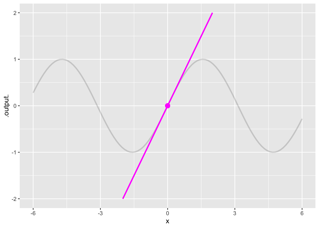

Draw your own graph of a sinusoid so that you can sketch on top of it the polynomial approximations you will design.
Start with sketching in a third-order polynomial that approximates the sinusoid near $x_0=0$. The general formula for a third order polynomial is \[\text{third}(x) \equiv \overbrace{\underbrace{b_0 + b_1 x^1}_\text{first-order polynomial} + b_2 x^2}^\text{second-order polynomial} + b_3 x^3\] To turn the first-order approximation into a third-order approximation algebraically, you would need to choose the coefficients $b_2$ and $b_3$. You want to choose the best possible $b_2$ and $b_3$ to stay close to the sinusoid. Of course, you could take the lazy person’s approach and choose $b_2 = b_3 = 0$. If you did that, you would have the first-order polynomial. Here’s the important point: the best third-order polynomial will not be any worse than the first-order polynomial, but it can be better!

Remember what you know about the shape of third-order polynomials:
1. One tail will go up, the other down.
2. There can be both an argmin and an argmax.
Repeat (1), sketching out a 5th-order polynomial. Again, one tail will go up and the other down. But now there can be two argmaxes and two argmins that alternate along the $x$ axis: min, max, min, max.
One more time, sketching now a 7th-order polynomial. Just like the first-, third-, and fifth-order polynomial, for the 7th one tail will go up and the other down. There can be as many as three argmaxes and three argmins. They will alternate: between any two argmaxes, there will be one argmin.

Exercise 11 We would like to write a Taylor-series polynomial for $\dnorm(x)$. To do this, we will need the folling numbers \[\dnorm(x_0),\ \ \partial_x \dnorm(x_0),\ \ \partial_{xx} \dnorm(x_0),\ \ \partial_{xxx} \dnorm(x_0), ...\]

(To warm up.) Why did I call the forms like $\partial_{xxx} \dnorm(x_0)$ a number rather than a function?

Because partial derivatives are numbers.

Because the notation $x_0$ is used to refer to a number, not the name of an input.

It was a mistake.

question id: birch-dig-radio-1

Here are the functions for the derivatives

Order	formula for derivative
0th	$\dnorm(x)$
1st	$\left({\large\strut}-x\right)\dnorm(x)$
2nd	$\left({\large\strut}x^2 - 1\right)\dnorm(x)$
3rd	$\left({\large\strut}3x - x^3\right)\dnorm(x)$
4th	$\left({\large\strut}3\,x^2-x^4 \right)\dnorm(x)$
5th	$\left({\large\strut}3-6\,x^3 + x^5 \right)\dnorm(x)$
6th	$\left({\large\strut}-15\,x^2 + 10\,x^4-x^6 \right)\dnorm(x)$
7th	$\left({\large\strut}-15 + 45\,x^3-15\,x^5 + x^7 \right)\dnorm(x)$
8th	$\left({\large\strut}105\,x^2-105\,x^4 + 21\,x^6-x^8 \right)\dnorm(x)$

Write a Taylor polynomial function for $\dnorm(x)$ around $x_0=0$). To do this, you will have to evaluate each of the 9 formulas above at $x=0$, producing a number. For example, the first five formulas will give 0.3989, 0, -0.3989, 0, 1.1968. This would expand into the Taylor function defined in Active R chunk 6:

Active R chunk 6

You will need to add in the 6th, 7th, and 8th terms.

Plot T_at_0(x) ~ x over the domain $0 \leq x \leq 2$, and pipe the result to a slice-plot of dnorm(x) ~ x so that you can compare the two plots.
Define another function T_at_1() which will be much like T_at_zero() but with x0=1 and the coefficients changed to be the formulas evaluated at $x=1$.
Add a layer showing T_at_1() to your previous plot.

Say over what domain T_at_0() is a good approximation to dnorm() and over what domain T_at_1() is a good approximation to dnorm(). Do the two domains overlap?

Write a piecewise function T() as defined in Active R chunk 7:

Active R chunk 7

Plot T() out on top of dnorm() to show whether T() is a good approximation to dnorm().

You could continue on to define T_at_2() and incorporate that into the piecewise T(), and so on, to construct an approximation to dnorm() that is accurate over a larger domain.

No answers yet collected

function	x⁰	x¹	x²	x³	x⁴	x⁵	x⁶	\(\cdots\)
\(e^x\)	+	+	+	+	+	+	+	\(\cdots\)
\(\cos(x)\)	+	0	-	0	+	0	-	\(\cdots\)
\(\sin(x)\)	0	+	0	-	0	+	0	\(\cdots\)
\(\ln(1+x)\)	0	+	-	+	-	+	-	\(\cdots\)