Chap 17 Exercises

$$$$

Loading webR...

Exercise 1 In this exercise, we ask you to estimate the slope from a graph of the function. But the function is exponential, so not a straight line.

A fundamental idea in calculus is that even a function with a curved graph will look like a straight line if you zoom in closely around a given point. And you know how to calculate the slope of a straight line.

When the graph is curved, the slope will be different at different points along the graph. So there is not a single slope for the function. Still, we can talk about the “slope at a point.”

One way to specify a point on a function’s graph is to give the horizontal coordinate: the input to the function. But here we will give you the output of the function. So long as the function passes the horizontal-line test, as the exponential does, specifying any particular output in the function’s range uniquely identifies a corresponding input.

Estimate the slope of the exponential function $g(x)\equiv e^x$ at several inputs, which we will call $x_1$, $x_2$, $x_3$ and $x_4$. We won’t give you numerical values for the $x_i$ points, but we will tell you the output of the function at each of those inputs. the values of $x$ where:

1. $g(x_1)=1$
2. $g(x_2)=5$
3. $g(x_3)=10$
4. $g(x_4)=0.1$

For each of (a)-(d), use Active R chunk 1 to plot the exponential function $e^x$ on a domain zoomed in around around the appropriate value of $x_i$. Then calculate the slope of the curve at that $x_i$.

Active R chunk 1

1

Using your answers for the slopes at the points given in (a)-(d), choose the best answer to this question: What is the pattern in the slope as $x$ varies?

The slope at each value $x_i$ is the same as $e^{x_i}$.

The slope at each value $x_i$ is the same as $x_i$.

The slope at each value of $x_i$ is the same as $x_i^2$.

The slope at each value of $x$ is the same as $\sqrt{x}.$

question id: exponential-slopes

Exercise 2  

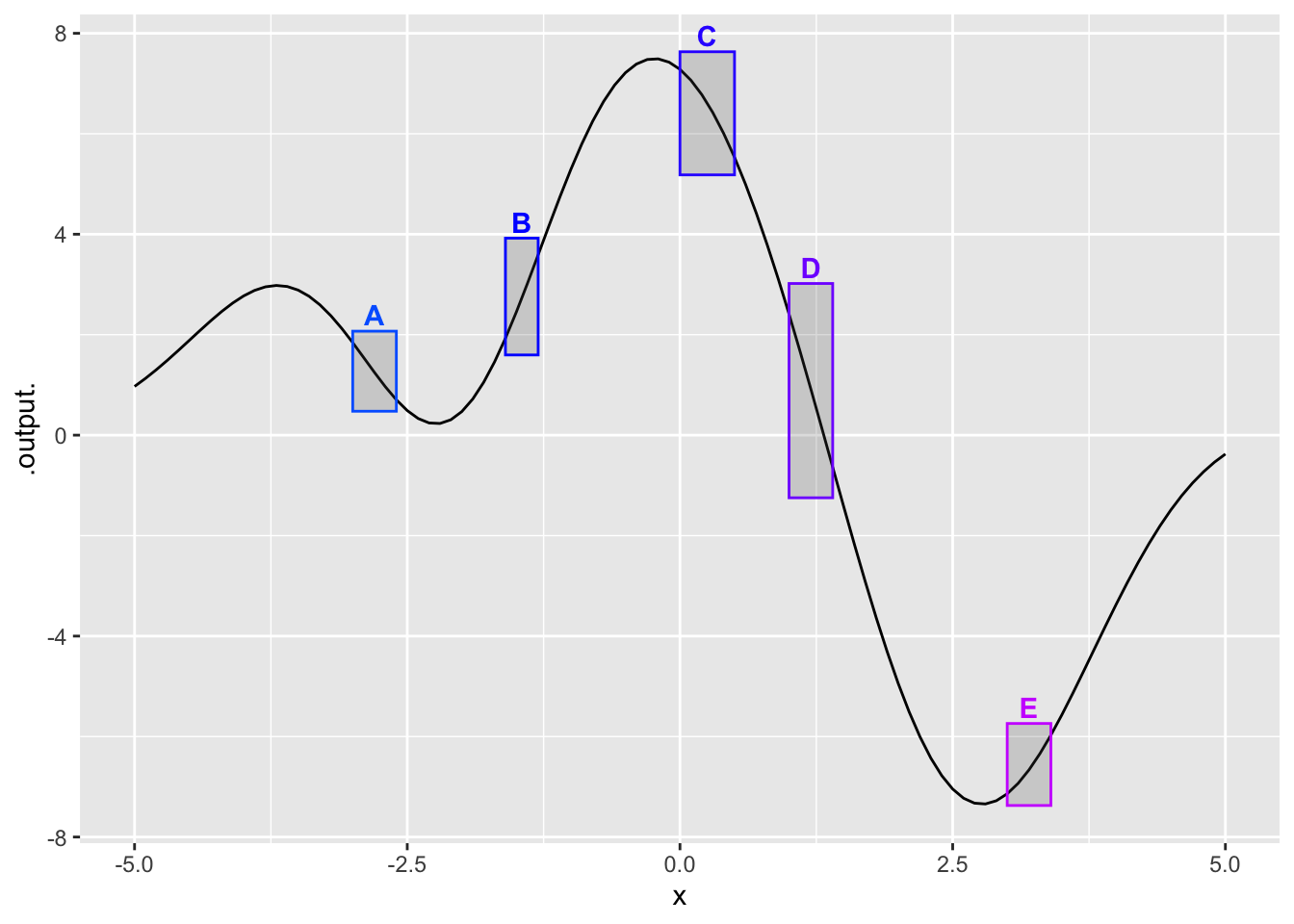
Glance at the graph. In which boxes is the slope negative?

A, B, C

B, C, D

A, C, D

question id: frog-bid-bed-1

Exercise 3  

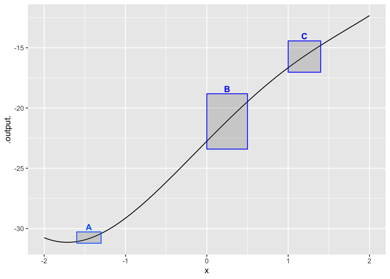
Figure 1

1. Consider the slope of the function in the domains marked by the boxes in Figure 1. What is the order of boxes from least steep to steepest?

A, B, C

C, A, B

A, C, B

none of these

question id: turtle-send-pot-1

Exercise 4 As you know, given a function $g(x)$ it is easy to construct a new function ${\mathcal{D}}_{x}g(x)$ that will be an approximation to the derivative ${\partial }_{x}g(x)$. The approximation function, which we call the slope function, can be $${\mathcal{D}}_{x}g(x)\equiv \frac{g(x+0.1)-g(x)}{0.1}$$

In Active R chunk 2, use makeFun() to create a function $g(x)\equiv e^x$ and another function called slope_of_g() using the definition of $\mathcal{D}g(x)$.

Active R chunk 2

1

2

g <- makeFun(exp(x) ~ x)

slope_of_g <- makeFun( _your_tilde_expression_here_ )

1. What’s the value of slope_of_g(1)?

0.37       0.85       1.37       1.85       2.85      

question id: wolf-talk-kayak-1

Using your sandbox, plot both g() and slope_of_g() (in blue) on a domain $-1\le x\le 1$. This can be done with slicePlot() in the following way:

Active R chunk 3

1

2

slice_plot(g(x) ~ x, domain(x = -1:1)) |>

  slice_plot(slope_of_g(x) ~ x, color = "blue")

2. Which of these statements best describes the graph of $g()$ compared to slope_of_g()?

slope_of_g() is negative compared to g(x).

slope_of_g() is shifted left by about $1$ compared to g(x).

slope_of_g() has a much smaller amplitude than g().

slope_of_g() is practically the same function as g(). That is, for any input the output of the two functions is practically the same.

question id: wolf-talk-kayak-2

17-exercises.rmarkdown

No answers yet collected