sq_wave <- makeFun(ifelse(abs(t) <= 0.5, 1, 0) ~ t)
slice_plot(sq_wave(t) ~ t, domain(t=-1:1))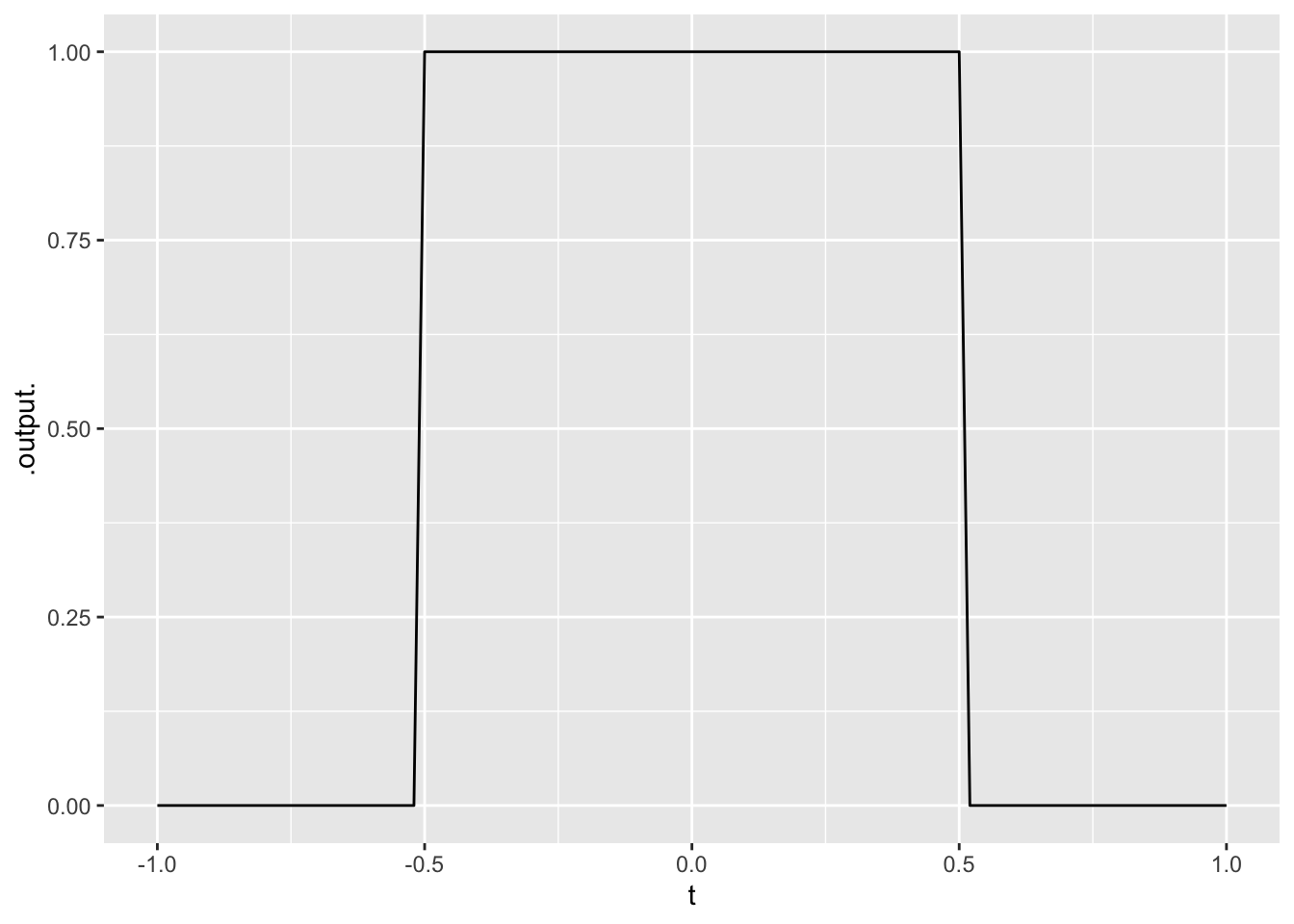
\[ \newcommand{\dnorm}{\text{dnorm}} \newcommand{\pnorm}{\text{pnorm}} \newcommand{\recip}{\text{recip}} \]
Exercise 1 Here is a square-wave function:
sq_wave <- makeFun(ifelse(abs(t) <= 0.5, 1, 0) ~ t)
slice_plot(sq_wave(t) ~ t, domain(t=-1:1))
Find the projection of the square wave onto each of these functions. Use the domain \(-1 \leq t \leq 1\).
Hint: To find the scalar multiplier of projecting \(g(t)\) onto \(f(t)\), use \[\int_{-1}^1 g(t)\, f(t)\, dt {\LARGE /} \int_{-1}^1 f(t)\, f(t)\,dt\] or, in R/mosaic
A <- Integrate(g(t)*f(t) ~ t, domain(t=-1:1)) /
  Integrate(f(t)*f(t) ~ t, domain(t=-1:1))
Then the projection of \(g()\) onto \(f()\) is \(A\, f(t)\).
Write down the scalar multiplier on each of the 8 functions above.
If you calculated things correctly, this is the linear combination of the 8 functions that best matches the square wave.
Loading required package: cubature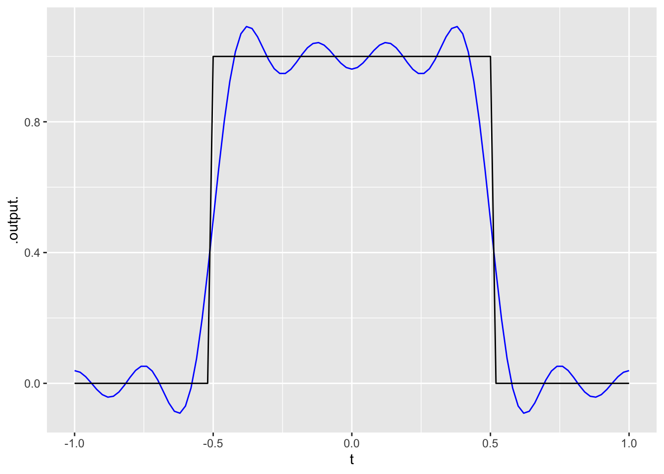
Exercise 2 Consider these functions/vectors on the domain \(0 \leq t \leq 1\):
Plot out each of the functions on the domain. How many complete cycles does each function complete as \(t\) goes from 0 to 1?
What is the length of each function?
All of the functions are mutually orthogonal except one. Which is the odd one out? (Hint: If the dot product is zero, the vectors are orthgonal.)
Exercise 3
Suppose we are interested in a domain \(0 \leq t \leq 10\) and a set of sinusoid functions:
\[s_1(t) \equiv \sin(2 \pi t/10)\\ s_2(t) \equiv \sin(4 \pi t/10)\\ s_3(t) \equiv \sin(6 \pi t/10)\\ c_1(t) \equiv \cos(2 \pi t/10)\\ c_2(t) \equiv \cos(4 \pi t/10)\\ c_3(t) \equiv \cos(6 \pi t/10) \]
Each of these functions goes through an integer number of cycles over \(0 \leq t \leq 10\), as you can confirm by graphing them, e.g.
s1 <- makeFun(sin(2*pi*t/10) ~ t)
s2 <- makeFun(sin(4*pi*t/10) ~ t)
# and so on
c2 <- makeFun(cos(4*pi*t/10) ~ t)
c3 <- makeFun(cos(6*pi*t/10) ~ t)
slice_plot(s1(t) ~ t, domain(t=0:10)) |>
  slice_plot(c2(t) ~ t, color="blue")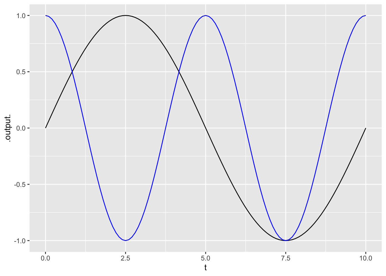
Using the definition of the dot product between two functions as \[f(t) \bullet g(t) \equiv \int_0^{10} f(t)\, g(t) dt\ ,\]
To simplify your calculations, you might want to make use of these “helper” functions:
fdot <- function(tilde1, tilde2, domain) {
  f <- makeFun(tilde1)
  g <- makeFun(tilde2)
  Integrate(f(t)*g(t) ~ t, domain)
}
fangle <- function(tilde1, tilde2, domain) {
  fdot(tilde1, tilde2, domain) /
    sqrt(fdot(tilde1, tilde1, domain) *
         fdot(tilde2, tilde2, domain))
}Exercise 4 (Still in draft. Figure out a nice activity based on this.)
id: anchorage-tides
Anchorage, AK
Components: - M2 12.42 hours - S2 12 hours - N2 12.658 hours - K1 23.935 hours
hour <- with(Anchorage_tide, hour)
b    <- with(Anchorage_tide, level)
sin1 <- sin(2*pi*hour/12.42)
cos1 <- cos(2*pi*hour/12.42)
sin2 <- sin(2*pi*hour/23.935)
cos2 <- cos(2*pi*hour/23.935)
sin3 <- sin(2*pi*hour/12)
cos3 <- cos(2*pi*hour/12)
sin4 <- sin(2*pi*hour/12.658)
cos4 <- cos(2*pi*hour/12.658)
A <- cbind(1, sin1, cos1, sin2, cos2, sin3, cos3, sin4, cos4)
mod1 <- b %onto% cbind(1, sin1, cos1)
mod2 <- b %onto% cbind(1, sin1, cos1, sin2, cos2)
x <- qr.solve(A, b)
mod3 <- A %*% x
resid <- b - mod3
gf_line(level ~ hour, data = Anchorage_tide)  %>%
  gf_line(mod3 ~ hour, color="magenta") %>%
  gf_lims(x = c(0,1000))
Warning: Removed 75114 rows containing missing values (`geom_line()`).
Removed 75114 rows containing missing values (`geom_line()`).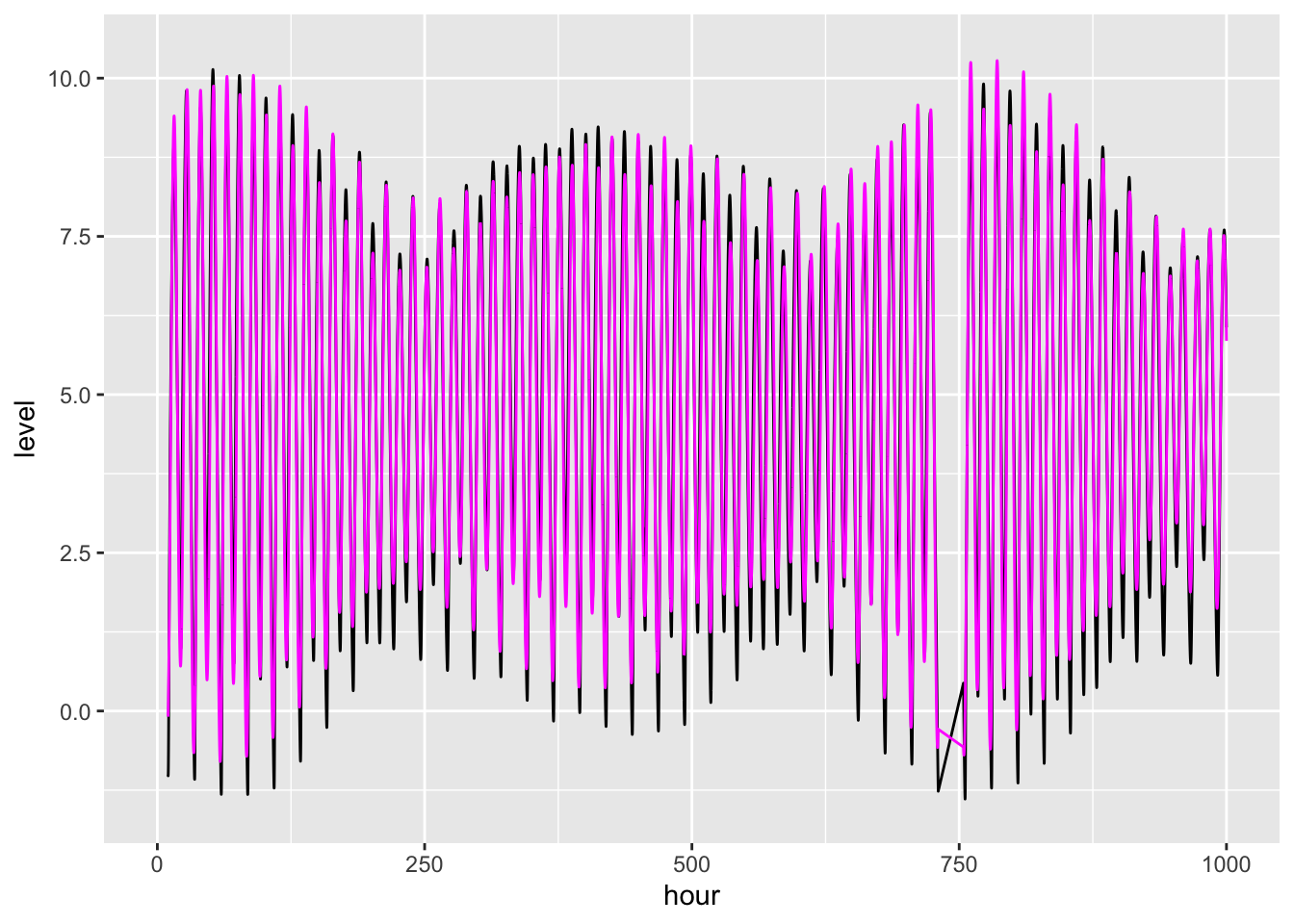
gf_line(resid ~ hour)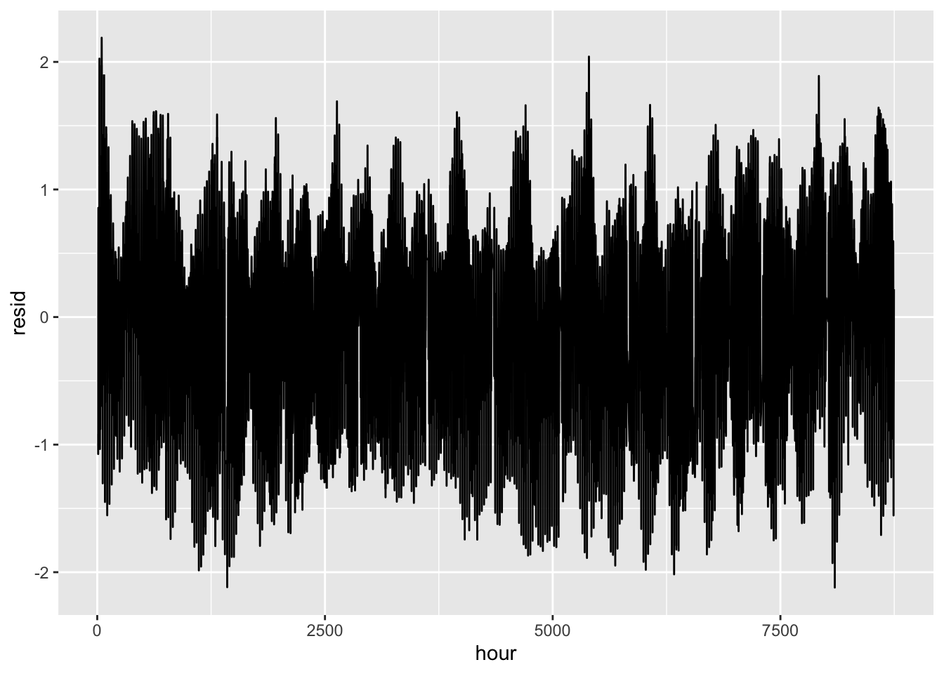
:::