Chap 4 Review

$$$$

Loading webR...

Figure 1: Contour plot of a function for the following three drill exercises.

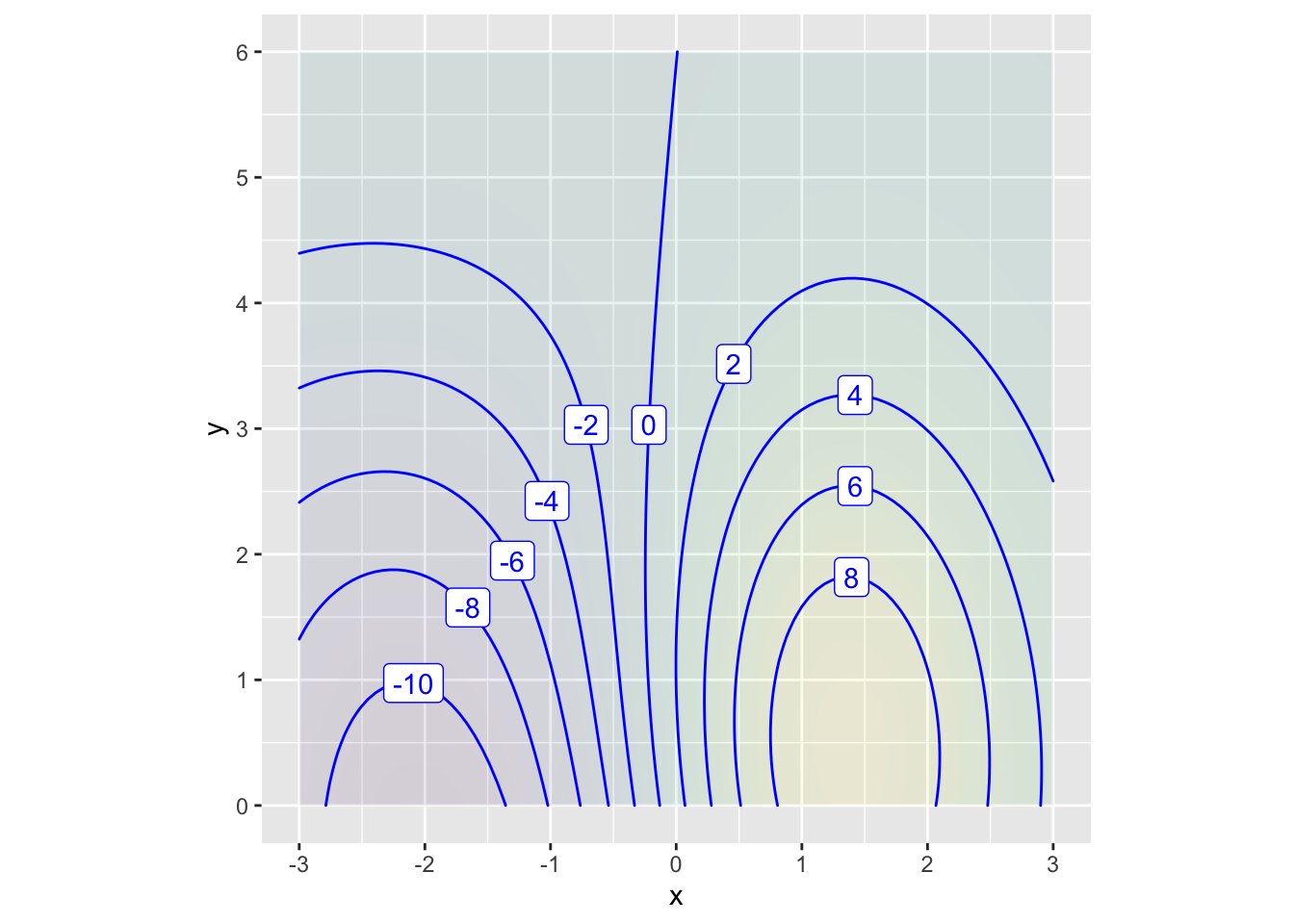
Exercise 1 Considering the function shown in Figure fig-drill-rev2-01, at which of these inputs is the function output nearly zero?

$(x=0,y=6)$

$(x=1,y=5)$

$(x=-2,y=6)$

$(x=0,y=1)$

question id: drill-Quiz-2-9

Exercise 2 Considering the function shown in Figure fig-drill-rev2-01, at which of these inputs is the function output nearly 1?

$(x=0,y=6)$

$(x=1,y=5)$

$(x=-2,y=6)$

$(x=0,y=1)$

question id: drill-Quiz-2-10

Exercise 3 Considering the function shown in Figure fig-drill-rev2-01, at which of these inputs is the function output nearly zero?

$(x=0,y=6)$

$(x=1,y=5)$

$(x=-2,y=6)$

$(x=0,y=1)$

question id: rX4ZzL

Exercise 4 Which of these is a positive-going zero crossing of $g(t)$ where $$g(t)\equiv \sin (\frac{2\pi }{5}t-3)?$$

$t=15/2\pi$       $t=2\pi /15$       $t=3$       None of the above      

question id: drill-Quiz-2-11

Exercise 5 Which of the following input values corresponds to a positive-going zero crossing of $g(t)$? $$\sin (\frac{2\pi }{5}(t-3))$$

$t=-5$       $t=-3$       $t=0$       $t=3$       $t=5$      

question id: drill-Quiz-2-14

Figure 2: Slice plot of a function for the following drill exercise.

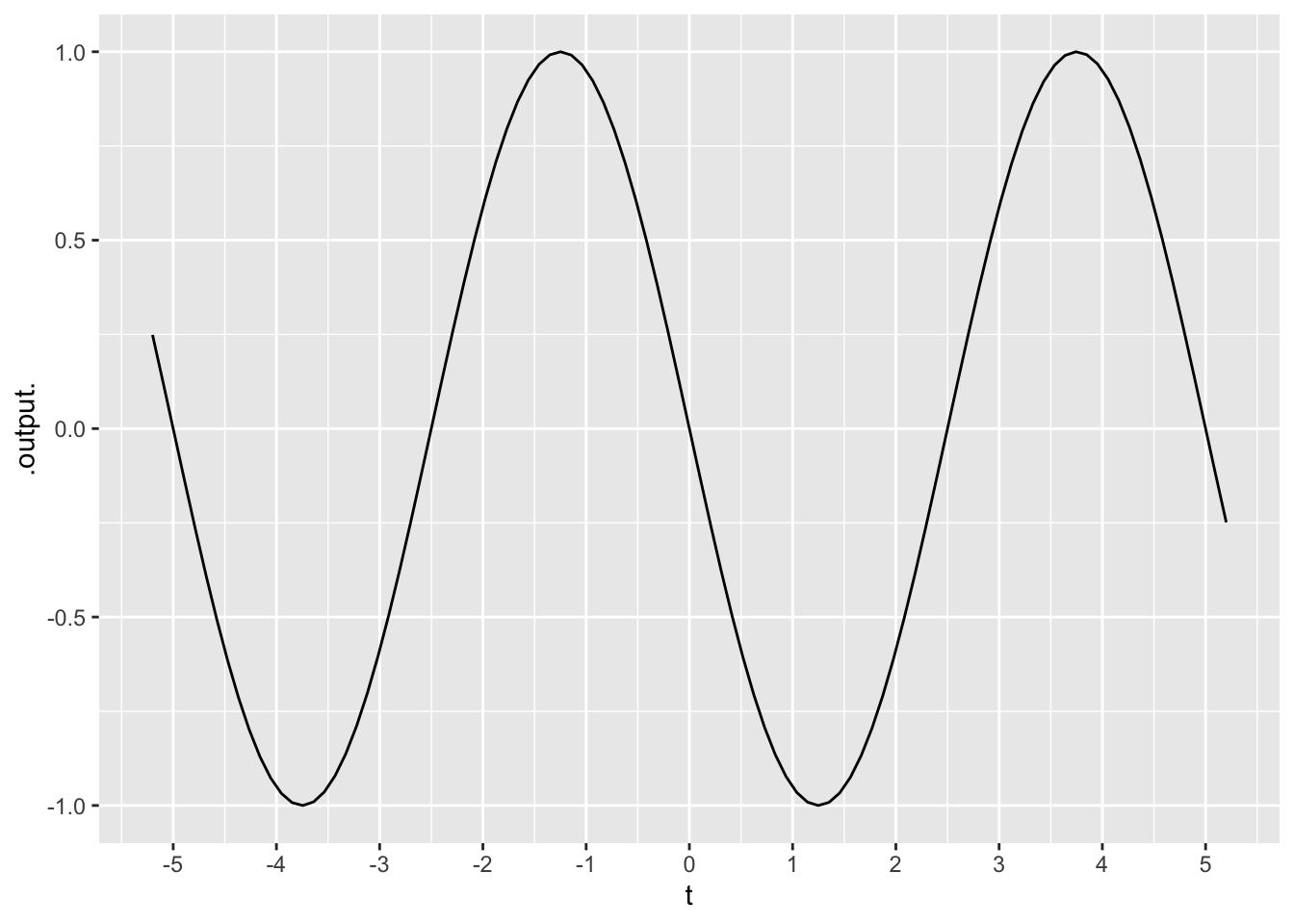
Exercise 6 Which input value is a negative-going zero-crossing of the function graphed in Figure fig-rev2-02?

$t=-2.5$       $t=-1.25$       $t=0$       $t=1.25$       $t=2.5$      

question id: drill-Quiz-2-2

slice_plot(sin(2*pi*t/5) ~ t, domain(t = -5.2 : 5.2)) |>
  gf_refine(scale_x_continuous(breaks = -5:5))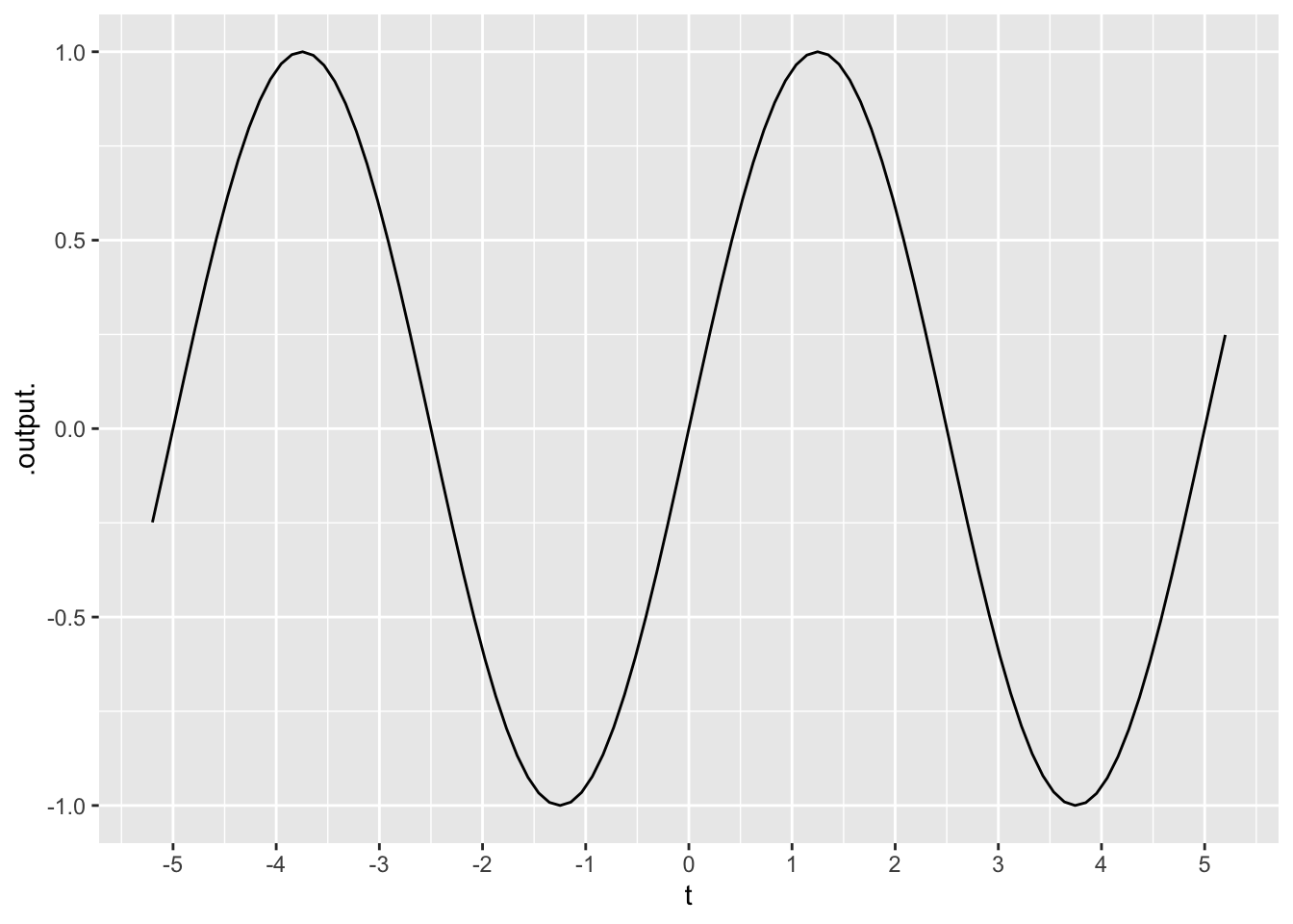

Figure 3: Slice plot of a function for the following drill exercise.

Exercise 7 Which input value is a positive-going zero-crossing of the function graphed in Figure fig-rev2-01?

$t=-5$       $t=-2.5$       $t=-1.25$       $t=1.25$       $t=2.5$      

question id: drill-Quiz-2-1

Figure 4: Contour plot of a function for the following three drill exercises.

Exercise 8 Considering the function graphed in Figure fig-drill-rev2-05, at which of these inputs is the function output nearly $-1$?

$(x=0,y=6)$

$(x=1,y=5)$

$(x=-2,y=6)$

$(x=0,y=1)$

question id: drill-Quiz-2-17

Figure 5: Contour plot of a function for the following drill exercise.

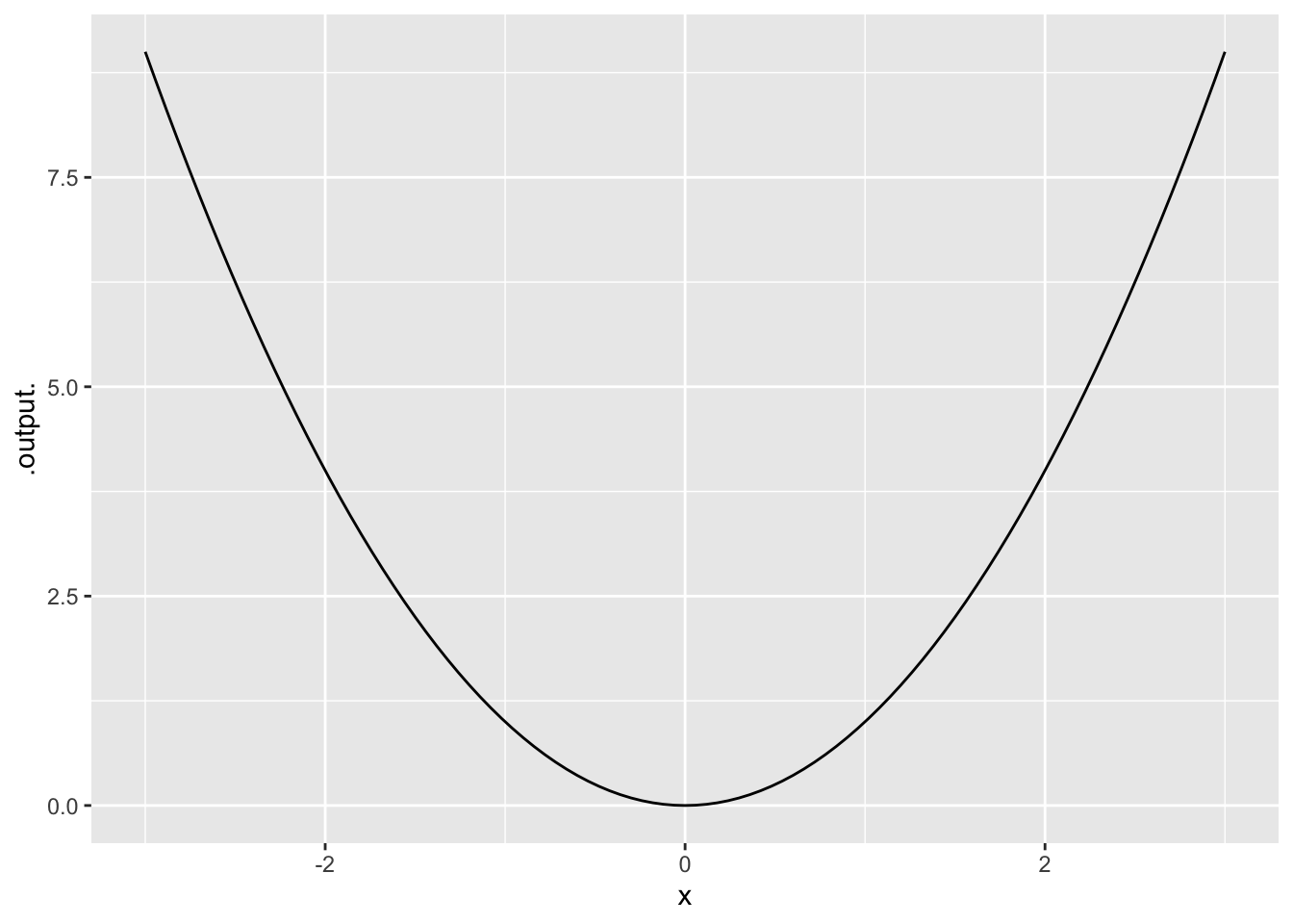
Exercise 9 Which command made this plot in Figure fig-M3-14-05?

slice_plot(x^2 ~ x, domain(x = -3 : 3))

plot(x^2 ~ x, domain= -3 : 3)

slice_plot(x^2, domain(x= -3 : 3))

slice_plot(x^2 ~ x, x= -3 : 3)

None of them correspond to the plot.

question id: drill-M04-29

Figure 6: .

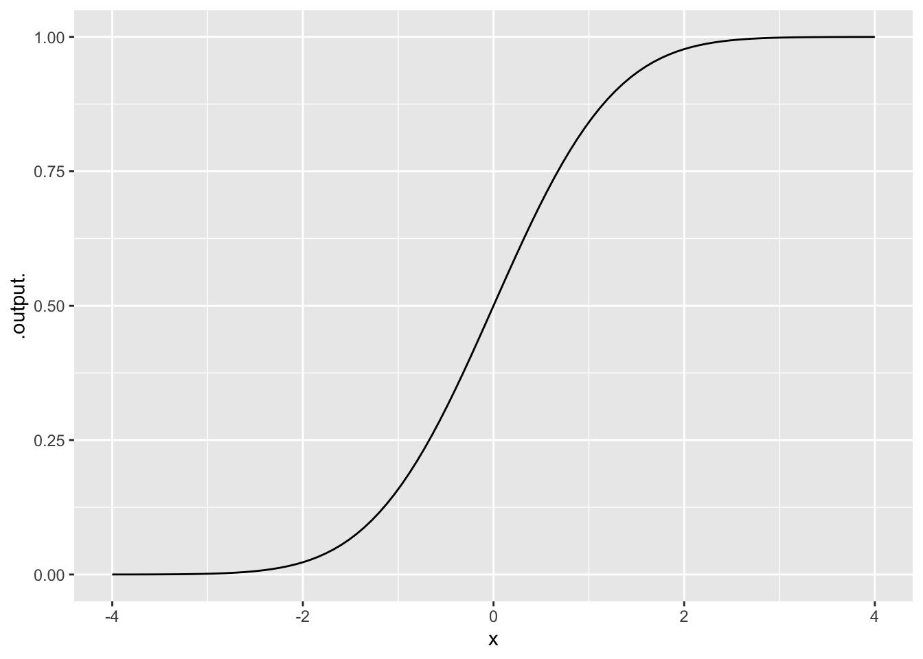
Exercise 10 Which command made the plot in Figure fig-M3-14-04?

slice_plot(pnorm(x) ~ x, domain(x = -4 : 4))

slice_plot(pnorm(x) ~ x, domain(x = -4 to 4))

slice_plot(pnorm(x) ~ y, domain(x = -4 : 4))

None of them correspond to the plot.

question id: drill-M04-30

Exercise 11 Only one of the following commands will successfully generate the graph of a function. Which one?

slice_plot(exp(y) ~ y, domain(y = -4, : 4))

slice_plot(pnorm(x) ~ x, domain(y = -4, 4))

slice_plot(log(x) ~ x, domain(x = 0 ; 10))

slice_plot(dnorm(y)) ~ x, domain(y = -3 : 3))

question id: drill-M04-31

04-review.rmarkdown

No answers yet collected