Chap 21 Exercises
\[ \newcommand{\dnorm}{\text{dnorm}} \newcommand{\pnorm}{\text{pnorm}} \newcommand{\recip}{\text{recip}} \]
Exercise 1
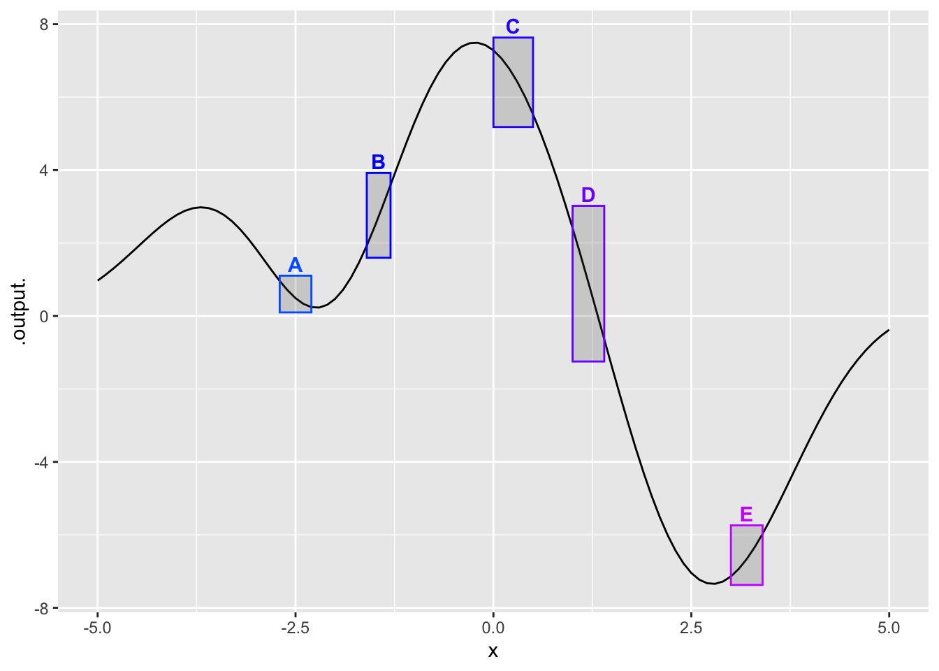
In which of the boxes is the function concave up?
A and E
B and D
C and D
question id: seahorse-speak-saucer-1
`
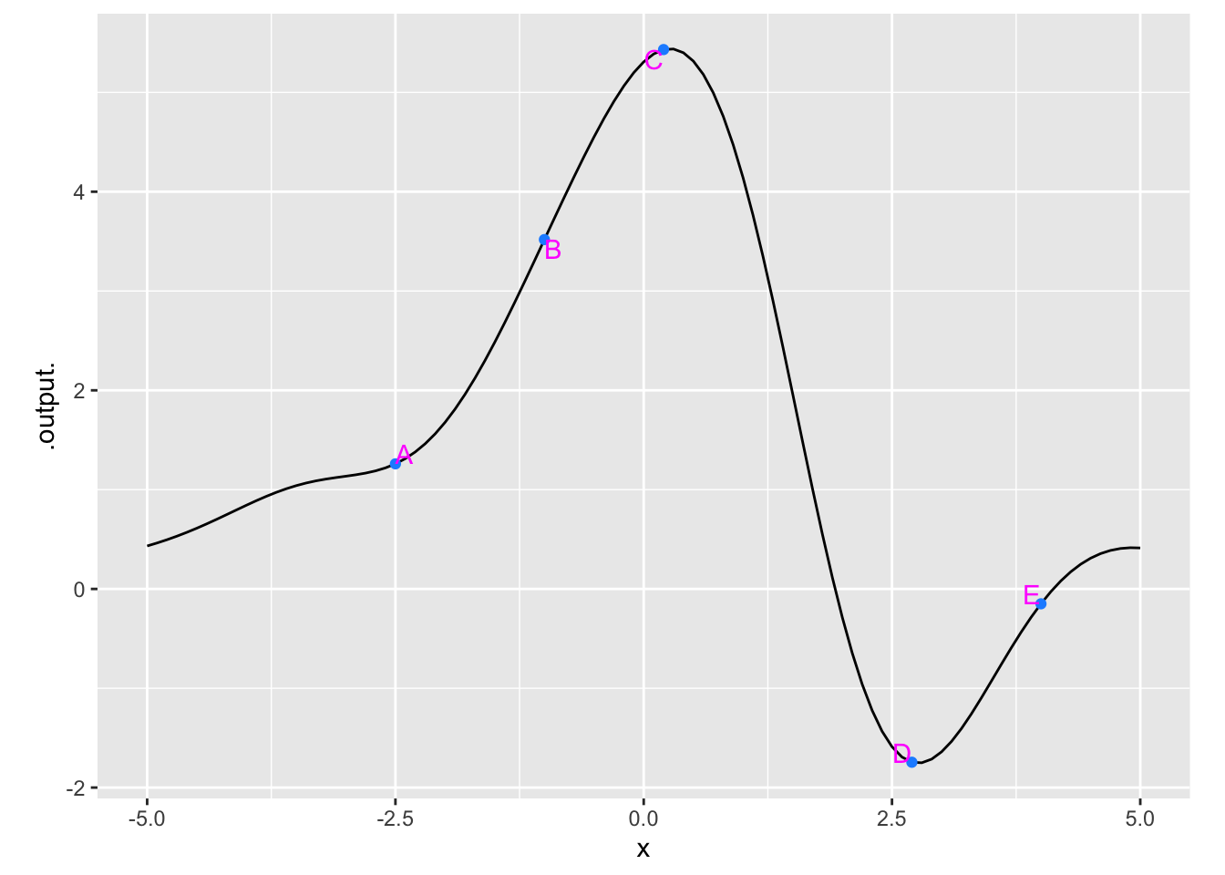
Exercise 2 Here is a smooth function marked at a few points. Your task is, at each point, to estimate the value of the derivative, the sign of the second derivative, and the radius of the circle that would nicely match the function in a small region around each point. (Remember, we are asking for the radius of the circle, which is half the diameter.)
To simplify things, here is a table giving seven different combinations of the quantities you are to estimate. Some of them correctly match one of the labeled points, some do not. All you need to do is choose which is the correct set of quantities for each labeled point.
| row | value of 1st deriv | sign of 2nd deriv | radius |
|---|---|---|---|
| i | -0.3 | pos | 0.25 |
| ii | 2.1 | near 0 | 2000 |
| iii | -1.4 | neg | 12 |
| iv | 0.3 | neg | 0.3 |
| v | 2.1 | pos | 0.1 |
| vi | 1.3 | neg | 3 |
| vii | 0.5 | pos | 1 |
- Which row from the table best matches the function at point A?
question id: daily-digital-26-QA5
- Which row from the table best matches the function at point B?
question id: daily-digital-26-QA6
- Which row from the table best matches the function at point C?
question id: daily-digital-26-QA7
- Which row from the table best matches the function at point D?
question id: daily-digital-26-QA8
- Which row from the table best matches the function at point E?
question id: daily-digital-26-QA9
Exercise 3
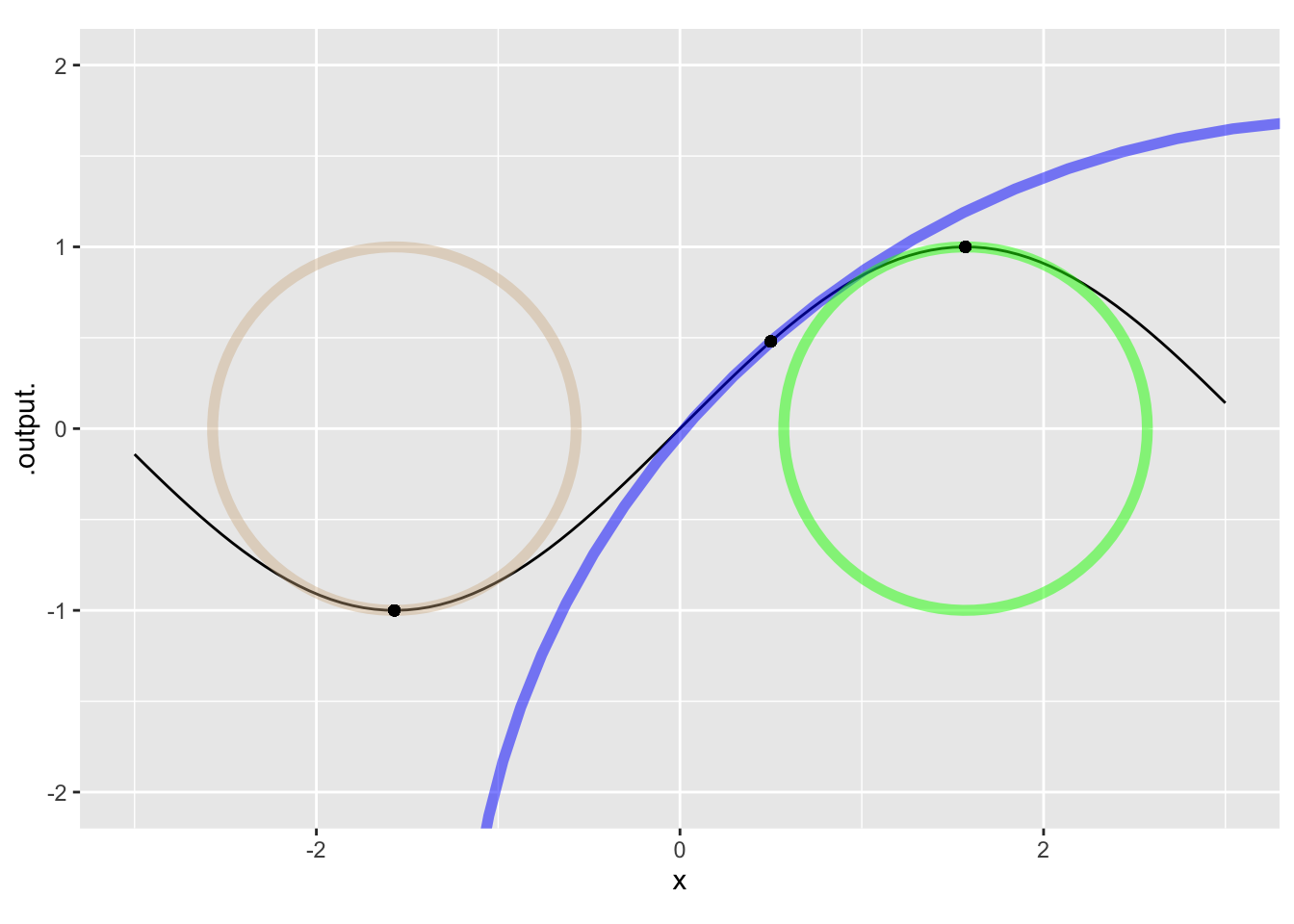
Calculate the curvature \(\cal K\) at each of the three input values marked in Figure 2. Do this by calculating the first and second derivatives of the sine function, evaluating those derivatives at the input values, and plugging them in to the formula in MOSAIC Calculus Sec 21.3.
- What is the curvature \(\cal K\) of \(\sin(x=-\pi/2)\)?
question id: chicken-sleep-knife-1
- What is the curvature \(\cal K\) of \(\sin(x=-0.923)\)?
question id: chicken-sleep-knife-2
- What is the curvature \(\cal K\) of \(\sin(x=\pi/2)\)?
question id: chicken-sleep-knife-3
- What is the curvature \(\cal K\) of \(\sin(x=0)\)? (Hint: You can tell straight from the graph, even though no enscribed circle has been drawn.
question id: chicken-sleep-knife-4
Exercise 4
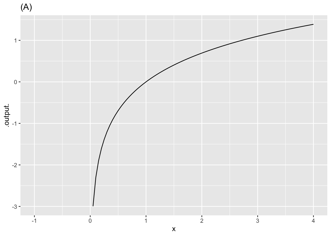
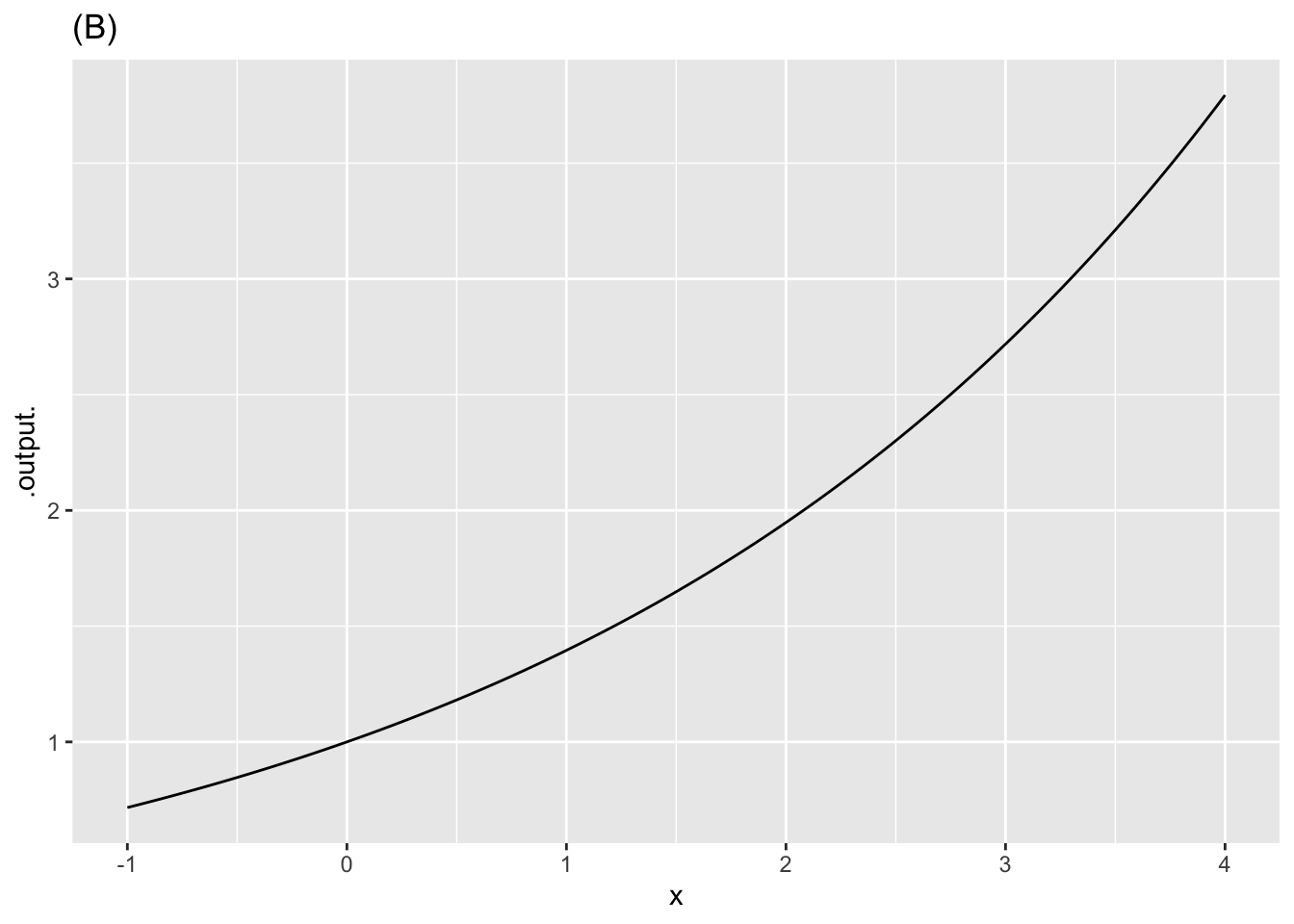
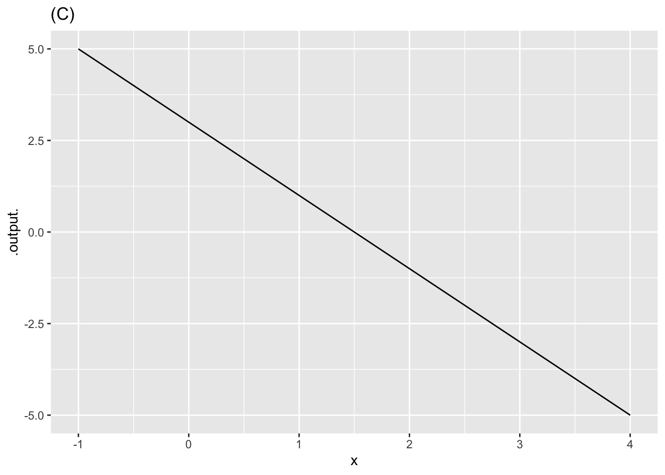
- Function (A) is
question id: concavity-1
- Function (B) is
question id: concavity-2
- Function (C) is
question id: concavity-3
- The negative of function (A) is
question id: concavity-4
Exercise 5
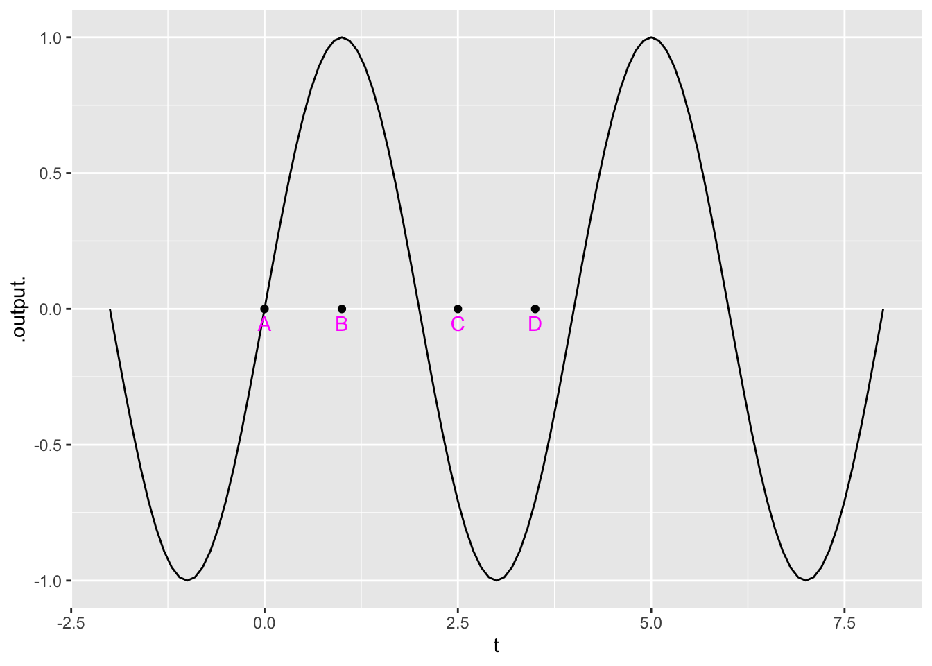
- For what values of the input \(t\) is the function in Figure 4 concave up?
question id: concavity-6
- For what values of the input \(t\) is the function in Figure 4 non-concave?
question id: concavity-8
- Where is the function in Figure 4 steepest?
question id: concavity-9
Exercise 6 We introduced concavity graphically and used the terms “concave up” and “concave down.” Now we can compute the concavity quantitatively using the second derivative.
Active R chunk 1 creates a random function f() and plot its. (Note: doodle_fun() generates random functions in the same way you might by moving a pencil smoothly on a piece of paper. The seed = 8427 effectively chooses which one of infinitely many functions is being generated. Different seeds give different functions. )
You can see that in the region near \(x = -1\) the function is concave down. While near \(x=2.5\) the function is concave up.
Active R chunk 2 computes the second derivative of \(f(x)\) and evaluate sit at \(x=-1\) and \(x=2.5\).
Using these results, and perhaps experimenting a little with different values of \(x\), you should be able to answer this question:
A. Which of these is a correct statement of “concave up” in terms of the value of \(\partial_{xx} f(x)\)?
A function is concave-up at input \(x_0\) when \(\partial_{xx} f(x_0) > 0\)
A function is concave-up at input \(x_0\) when \(\partial_{xx} f(x_0) < 0\)
A function is concave-up at input \(x_0\) when \(\partial_{xx} f(x_0) < 0\) and \(\partial_x f(x_0) < 0\)
A function is concave-up at input \(x_0\) when \(\partial_{xx} f(x_0) > 0\) and \(\partial_x f(x_0) > 0\)
question id: crow-write-chair-A
Recall that an inflection point is a value for the input \(x\) at which \(f(x)\) changes from concave up to concave down, or vice versa. Add a statement to Active R chunk 2 to graph \(\partial_{xx} f(x)\).
B. From reading the graph of \(\partial_{xx} f(x)\), say which of these is nearest to an inflection point for \(f(x)\).
question id: crow-write-chair-B
C. How many inflection points are there for \(f(x)\) in the domain \(-5 \leq x \leq 5\)?
question id: crow-write-chair-C
Exercise 7 The function road(x) has been constructed to correspond to a curved road of gradually tighter radius from left to right
Using Active R chunk 3, calculate the curvature of this road for each value of \(x\).
- What is the curvature of the road at \(x=-1\)?
question id: tiger-blow-futon-1
- What is the curvature of the road at \(x=1\)?
question id: tiger-blow-futon-2
- What is the curvature of the road at \(x=0\)?
question id: tiger-blow-futon-3
Exercise 8 The graph of the function \(g(x) \equiv \sqrt{\strut R^2 - x^2}\) has the shape of a semi-circle of radius \(R\), e.g.
g <- makeFun(sqrt(R^2 - x^2) ~ x, R = 2)
slice_plot(g(x) ~ x, domain(x = -2:2), npts=300)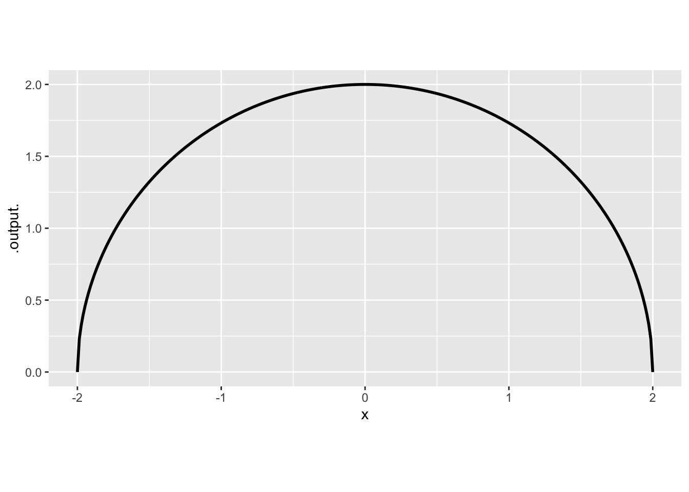
Intuition suggests that the radius of an enscribed circle for \(g()\) should match the radius of the graph of the function.
Using Active R chunk 4, create a function to calculate the curvature of \(g()\) at any input \(x\). Then plot that curvature function over the domain \(-2 < x < 2\). Is the curvature of \(g()\) indeed constant? To help you get started, here is some R/mosaic code with a fill-in-the-blank for the formula.
For instance, let’s set the default value of the parameter \(R\) to be 2.
What is the curvature of \(g(x)\)?
question id: goat-come-bed-1
Activities
Exercise 9 Pilots of commercial passenger aircraft consider the comfort of their passengers into account when flying. In transitioning from level flight onto the descent path for landing, for example, pilots take care that the vertical component of acceleration isn’t so great that passengers feel the plane “falling out from under them.”
A simple model of the descent path is a sigmoid function. Suppose that the descent starts from an altitude of \(A = 20,000\) feet at a distance of 30,000 feet from the end of the runway. A reasonable model for the vertical component of the flight path is \[\text{altitude}(x) \equiv A\,\pnorm(x,\ \ mn=30000/2,\ \ sd=30000/6)\] Notice that the parameter “mean” is set to be half the distance to the runway, and the parameter “sd” is set to be a third of that. This ensures that the start and end of the descent will involve flight that is close to level.
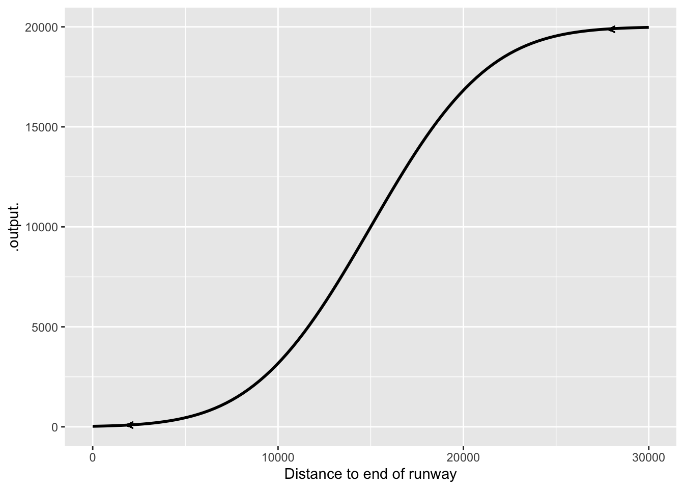
The vertical acceleration is the second derivative of altitude() with respect to time: \(\partial_{tt} \text{altitude}(t)\). But notice that altitude() is a function of distance from the runway, not time.
To treat altitude() as a function of time, we need to write “distance from the runway” as a function of time. Let’s set \(t=0\) to be the time when the plane begins its descent, when it is 30,000 feet from the end of the runway. Distance from the runway will be \[x(t) = 30000 - v\, t\] where \(v\) is the plane’s velocity. Composing altitude() onto \(x(t)\) gives a new function \[\text{alt}(t) \equiv \text{altitude}(x(t)) = \text{altitude}(30000-v\, t)\]
Suppose that the aircraft is flying at \(v = 200\) miles-per-hour, which is \[200 \frac{\bcancel{\text{miles}}}{\cancel{\text{hour}}} \frac{\cancel{1\, \text{hour}}}{3600\, \text{s}} \frac{5280 \text{ft}}{\bcancel{1\, \text{mile}}} = 293.3 \frac{\text{ft}}{\text{s}}\]. At that speed, it will take a little more than 100 seconds for the aircraft to reach the runway.
In Active R chunk 5 plot out the function alt(\(t\)) function, choosing a domain for \(t\) that lets you see the whole descent path.
Compute the second derivative \(\partial_{tt} \text{alt}(t)\) to find the vertical component of acceleration of the aircraft. (Important note: Due to a bug in R/mosaic, use numD() rather than D() to compute the second derivative.)
Graph the second derivative over the appropriate domain and look for the most extreme values of acceleration.
- From the graph, read off the maximum vertical acceleration during the descent.
What are the units of vertical acceleration shown in the graph?
question id: descent-path-1
A rule of thumb is that a vertical acceleration up to \(5\, \text{ft}\, \text{s}^{-2}\) is acceptable in terms of passenger comfort. Regrettably, the descent path we described does not meet the standard! So we have to re-design the descent path. Since both the altitude and velocity are set, the only parameter you can change is the distance from the foot of the runway where descent commences. Of course, for the parameters “mean” and “sd” need to be set accordingly.
- What are the units of vertical acceleration shown in the graph?
feet-per-second
feet-per-second-squared
miles-per-hour-squared
question id: descent-path-2
For reflection: A new hire at the airline’s operations center proposes to model the descent as a straight-line function rather than a sigmoid. He points out that the second derivative of a straight-line function is always 0, so the passengers would feel no acceleration at all! Explain to this newbie what’s wrong with his idea.
Exercise 10
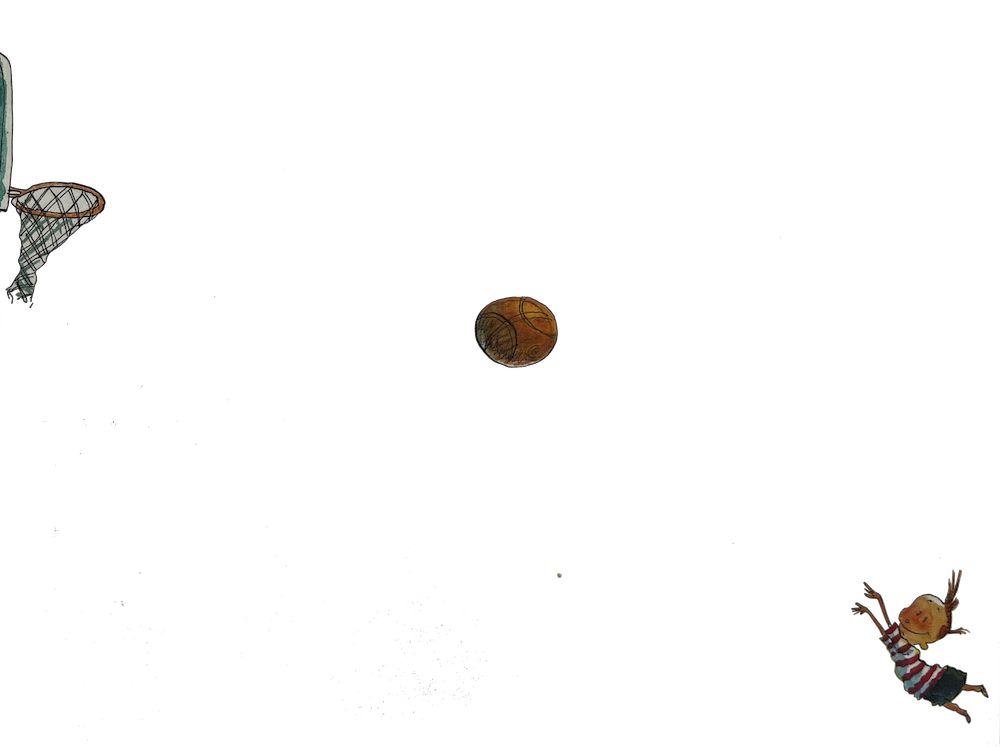
The picture in Figure 6 shows an instantaneous position of the ball. However, such a snapshot does not show the instantaneous velocity of the ball. If you had a few frames of a movie, your intuition would tell you if the ball is likely to go through the hoop. From a movie, you could even calculate a good finite-difference approximation to the instantaneous velocity of the ball. (In Block VI, you’ll see how to use the instantaneous position and velocity to trace out the trajectory of the ball up to the moment it comes into contact with the basket, hoop, or backboard.)
Assume for the purposes of the following question that the boy, the center of the ball, and the center of the hoop are all in the same plane, as required for a swish shot. Assume as well that when the ball left the boy’s hands it was in the position now occupied by the boy’s head and that there was no spin on the ball. Now the question:
Will the ball swish through the basket?
Use calculus concepts to make a good argument about whether the answer should be “impossible” or “possible.”
Think of the path of the ball as a function \(f(x)\), where \(x\) is position along the floor and \(f(x)\) gives the corresponding height of the ball. Draw some intuitively plausible paths. That is, draw graphs of possible functions consistent with the picture and with the assumption that the launch point is marked by the current position of the boy’s head.
From the picture you can easily find the line connecting the ball’s current position with the launch point. The slope of this line is the average rate of change of ball height with respect to \(x\).
The physics of ball flight (with no spin) requires the function \(f(x)\) to be concave down. How does this restrict the set of possible paths?