32 Statistical modeling and R²

So far, we’ve been looking at linear combinations from a distinctively mathematical point of view: vectors, collections of vectors (matrices), projection, angles and orthogonality. We’ve show a few applications of the techniques for working with linear combinations, but have always expressed those techniques using mathematical terminology. In this Chapter, we will take a detour to get a sense of the perspective and terminology of another field: statistics.

In the quantitative world, including fields such as biology and genetics, the social sciences, business decision making, etc. there are far more people working with linear combinations with a statistical eye than there are people working with the mathematical form of notation. Statistics is a far wider field than linear combination, so this chapter is not an attempt to replace the need to study statistics and data science. The purpose is merely to show you how a mathematical process can be used as part of a broader framework to provide useful information to decision-makers.

Since a statistics and data-science courses are part of a complete quantitative education, we want to point out from the beginning what you are likely to experience a traditional introductory statistics course and why that will seem largely disconnected from what you see here.

Statistics did not start as a branch of mathematics, although people trained as mathematicians played a central role in its development. The story is complicated, but a simplification faithful to that history is to see statistics as an extension of biology. Statistics emerged in the last couple of decades of the 1800s. Possibly the key motivation was to understand genetics and Darwinian evolution. Today we know much about DNA sequences, RNA, amino acids, proteins, and so on. But quantitative genetics started in complete ignorance of any physical mechanism for genetics. Instead, mathematical models were the basis for the theory of genetics, beginning with with Gregor Mendel’s work on heritable traits published in 1865.¹

Perhaps coincidentally—or perhaps not—Charles Darwin (1809-1882) was a half-cousin of Francis Galton (1822-1911). Traditional introductory statistics is based, more or less, on the work Galton and his contemporaries, for instance Karl Pearson (1857-1936) and William Sealy Gosset (1876-1937). The terms that you encounter in introductory statistics—correlation coefficient, regression, chi-squared test, t-test—where in place by 1910. Ronald Fisher (1890-1962), also a geneticist, extended this work based in part on the mathematical ideas of projection. Fisher invented analysis of variance (ANOVA) and maximum likelihood estimation and is perhaps the “great man” of statistics. (See Section 35.004 for an introduction to likelihood. We will briefly touch on ANOVA in this chapter.) To his historical discredit, Fisher was a leader in eugenics. He was also a major obstacle, to the statistical acceptance of the dangers of smoking.

Most of the many techniques covered in traditional introductory statistics are, in fact, manifestations of the application of a general technique: the target problem. They are not taught this way, partly out of hide-bound tradition and partly because the target problem has been covered, if at all, in the fourth or fifth semester of a traditional calculus sequence.

It often happens that a model is needed to help organize complex, multivariate data for purposes such as prediction. As a case in point, consider the data available in the Body_fat data frame, which consists of measurements of characteristics such as height, weight, chest circumference, and body fat on 252 men.

bodyfat	age	weight	height	neck	chest	abdomen	hip	thigh	knee	ankle	biceps	forearm	wrist
12.3	23	154.25	67.75	36.2	93.1	85.2	94.5	59.0	37.3	21.9	32.0	27.4	17.1
6.1	22	173.25	72.25	38.5	93.6	83.0	98.7	58.7	37.3	23.4	30.5	28.9	18.2
25.3	22	154.00	66.25	34.0	95.8	87.9	99.2	59.6	38.9	24.0	28.8	25.2	16.6
... 252 rows in total ...
26.0	72	190.75	70.5	38.9	108.3	101.3	97.8	56.0	41.6	22.7	30.5	29.4	19.8
31.9	74	207.50	70.0	40.8	112.4	108.5	107.1	59.3	42.2	24.6	33.7	30.0	20.9

Body fat, the percentage of total body mass consisting of fat, is thought by some to be a good measure of general fitness. To what extent this theory is merely a reflection of general societal attitudes toward body shape is unknown.

Whatever its actual utility, body fat is hard to measure directly; it involves submerging a person in water to measure total body volume, then calculating the persons mass density and converting this to a reading of body-mass percentage. For those who would like to see body fat used more broadly as a measure of health and fitness, this elaborate procedure stands in the way. And so they seek easier ways to estimate body fat along the lines of the Body Mass Index (BMI), which is a simple arithmetic combination of easily measured height and weight. (Note that BMI is also controversial as anything other than a rough description of body shape. In particular, the label “overweight,” officially \(25 \leq \text{BMI}\leq 30\) has at best little connection to actual health.)

How can we construct a model, based on the available data, of body fat as a function of the easy-to-measure characteristics such as height and weight? You can anticipate that this will be a matter of applying what we know about the target problem

\[\text{Given}\ \mathit{A}\ \text{and}\ \vec{b}\text{, solve } \mathit{A} \vec{x} = \vec{b}\ \text{for}\ \vec{x}\]where \(\vec{b}\) is the column of body-mass measurements and \(\mathit{A}\) is the matrix of all the other columns in the data frame.

In statistics, the target \(\vec{b}\) is called the response variable and \(\mathit{A}\) is the set of explanatory variables. You can also think of the response variable as the output of the model we will build and the explanatory variables as the inputs to that model.

Although application of the target problem is an essential part of constructing a statistical model, it is far from the only part. For instance, statisticians find is useful to think about “how much” of the response variable is explained by the explanatory variables. Measuring this requires a definition for “how much.” In defining “how much,” statisticians focus not on how much variation there is among the values in the response variable. The standard way to measure this is with the variance, which was introduce in Section 28.4 and can be thought of as the average of pair-wise differences among the elements in \(\vec{b}\).

to support this focus on the variance of \(\vec{b}\), statisticians typically augment \(\vec{A}\) with a column of ones, which they call the intercept.

To move forward, we will extract the response variable from the data and construct \(\vec{A}\), adding in the vector of ones. We will show the vector/matrix commands for doing this, but you don’t have to remember them because statisticians have a more user-friendly interface to the calculations.

We will be constructing vectors and matrices from the columns of a data frame. You can do this with the R/mosaic function df2matrix() (the df stands for “data frame”). The final argument to df2matrix() is the name of the data frame. Previous arguments are the columns you want to insert in the matrix. We can make both b and A using df2matrix(). Note the 1 that is inserted as a column into A.

b <- df2matrix(bodyfat, data = Body_fat)
A <- df2matrix(1, wrist, thigh, forearm, data = Body_fat)

You can also include interaction terms (e.g. wrist*thigh) or transformations (e.g. log(forearm)) as columns in the A matrix.

Once we have b and A, we find the coefficients on the linear model in the usual way, with qr.solve().

x <- qr.solve(A, b)

Having applied qr.solve(), \(\vec{x}\) now contains the coefficients on the “best” linear combination of the columns in \(\vec{A}\). One of the ways in which the R language is designed to support statistics, is that it keeps track of names of columns, so the elements of \(\vec{x}\) are labelled with the name of the column the element applies to.

x
##             bodyfat
## 1       -40.4700038
## wrist     0.2533051
## thigh     0.8181824
## forearm   0.2232146

Based on the above, the model for body fat as a function of the explanatory variables is:

\[\text{body fat} = -40.5 + 0.253\, \mathtt{wrist} - 0.818\, \mathtt{thigh} - 0.223\, \mathtt{forearm}\ .\]

In invoking qr.solve(A, b) we have created a vector x containing the solution to the target problem. We can use that vector x in the usual ways, for example to construct the model vector (A %*% x) or the residual vector (b - A %*% x).

Sometimes you will want to create a function that implements the linear combination described by x. For convenience, the R/mosaic makeFun() knows how to accept a vector input and create the corresponding function. For example:

f <- makeFun(x)
f
## function (wrist, thigh, forearm) 
## -40.4700037897818 * 1 + 0.253305146981963 * wrist + 0.818182409571164 * 
##     thigh + 0.223214640718424 * forearm
## <environment: 0x7fd1b932eef0>

32.1 How good a model?

There are so many ways to construct a linear-combination model from a data frame—all the different combinations of columns plus possibly interaction terms and other transformations—that it is natural to ask, “What’s the best model?”

As always, “best” depends on the purpose for your model is to be used. This requires thought on the part of the modeler. One method you will often encounter is called R-squared and written R².

The basic question addressed by R² is: How much of the variation in the response variable b is accounted for by the columns of the matrix A. The standard way to measure the “amount of variation” in a variable is the variance. In R, you calculate that with

var(b)
##          bodyfat
## bodyfat 70.03582

We can also look at the variation in the model vector, \(\hat{b}\).

bhat <- A %*% x
var(bhat)
##          bodyfat
## bodyfat 22.16637

R² is simply the ratio of these two variances:

var(bhat) / var(b)
##           bodyfat
## bodyfat 0.3165004

This result, 31.7%, is interpreted as the fraction of the variance in the response variable that is accounted for by the model. Near synonyms for “accounted for” are “explained by” or “can be attributed to.”

In the same spirit, we can ask how much of the variance in the response variable is unexplained or unaccounted for by the explanatory variables . To answer this, look at the size of the residual:

var(b - bhat) / var(b)
##           bodyfat
## bodyfat 0.6834996

Notice that the amount of variance explained, 68.3%, plus the amount remaining unexplained, 31.7%, add up to 100%. This is no accident. The additivity is why statisticians use the variance as a measure of variability.

32.2 Machine learning

If you pay attention to trends, you will know about advances in artificial intelligence and the many claims—some hype, some not—about how it will change everything from animal husbandry to warfare. Services such as Google Translate are based on artificial intelligence, as are many surveillance technologies. (Whether the surveillance is for good or ill is a serious matter.)

Skills in artificial intelligence are currently a ticket to lucrative employment.

Like so many things, “artificial intelligence” is a branding term. In fact, what all the excitement is about is not mostly artificial intelligence at all. The advances, by and large, have come over 50 years of development in a field called “statistical learning” or “machine learning,” depending on whether the perspective is from statistics or computer science.

A major part of the mathematical foundation of statistical (or “machine”) learning is linear algebra. Many workers in “artificial intelligence” are struggling to catch up because they never took linear algebra in college or, if they did, they took a proof-oriented course that didn’t cover the elements of linear algebra that are directly applicable. We are trying to do better in this course.

So if you’re diligent, and continue your studies to take actual statistical/machine learning courses, you will find yourself at the top of the heap. Even xkcd, the beloved techno-comic, gets in on the act, as this cartoon reveals:

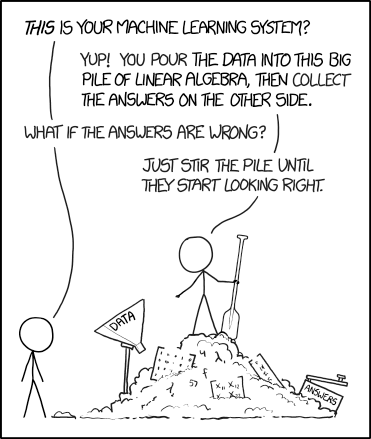
Look carefully below the paddle and you will see the Greek letter “lambda”, \(\lambda\). You will meet the linear algebra concept signified by \(\lambda\)—eigenvalues and eigenvectors—in Block 6.

We’ve been using the R/mosaic function df2matrix() to construct the A and b matrices used in linear model from data. This is mainly for convenience: we need a way to carry out the calculations that lets you see the x vector, and calculate the model vector and the residual in the way described in Chapter Chapter 31.

In practice, statistical modelers use other software. The most famous of these in R is the lm() family of functions. This does all the work of creating the b vector and the A matrix, QR solving, etc. We call it a “family” of functions because the output of lm() is not simply the vector of coefficients x but includes many other features that support statistical inference on the models created.

In a statistics course using R, you are very likely to encounter lm(). You will never hear about df2matrix() outside of this book.

32.3 Exercises

Exercise 32.01

A. What’s the largest possible value for R²?

As you know, R² is a ratio of variances. A good way to think of variance is as the square length of a vector. So think about R² as if it were calculated from the square length of \(\vec{b}\) and \(\hat{b}\).

(Hint: What does the projection problem tell you about the lengths of \(\vec{b}\) and \(\hat{b}\).)

B. What’s the smallest possible value for R²? (Hint: What’s the smallest possible length for \(\hat{b}\)?)

Amazingly, this work attracted little attention until after 1900, when Mendel’s laws were rediscovered by the botanists de Vries, Correns, and von Tschermak.↩︎