25 Partial change and the gradient vector
For a function with one input, the derivative function (with respect to that input) outputs a single quantity at each input value. We have often drawn the quantity as a sloping line. This is easy to do on the two-dimensional surface of paper or a screen.
It would be silly to restrict our models to using functions of a single variable just so that we can show them on paper or a screen. For functions with multiple inputs, the output of the derivative function will not be a single quantity, but a set of quantities, one for each input. The derivative of a function of multiple inputs with respect to only one of those inputs is called a partial derivative. “Partial” is a reasonable word here, because each partial derivative gives only part of the information about the overall derivative with respect to all of the inputs. The set of all the partial derivatives, called the gradient, is a way of representing the “slope” of a function of multiple inputs.
25.1 Calculus on two inputs
Although we use contour plots for good practical reasons, the graph of a function \(g(x,y)\) with two inputs is a surface, as depicted in Figure fig-first-surface. The derivative of \(g(x,y)\) should encode the information needed to approximate the surface at any input \((x,y)\). In particular, we want the derivative of \(g(x,y)\) to tell us the orientation of the tangent plane to the surface.
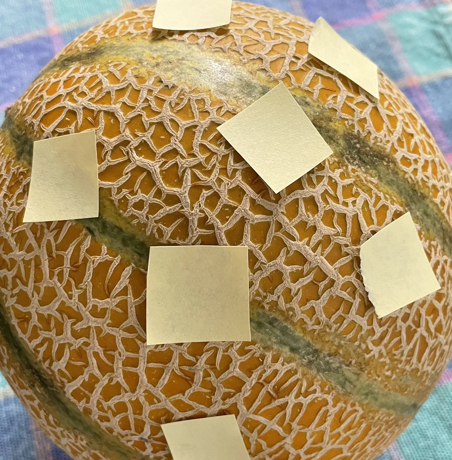
A tangent plane is infinite in extent. Let’s use the word facet to refer to a little patch of the tangent plane centered at the point of contact. Each facet is flat. (it is part of a plane!) Figure fig-melon-facets shows some facets tangent to a familiar curved surface. No two of the facets are oriented the same way.
Better than a picture of a summer melon, pick up a hardcover book and place it on a curved surface such as a basketball. The book cover is a flat surface: a facet. The orientation of the cover will match the orientation of the surface at the point of tangency. Change the orientation of the cover and you will find that the point of tangency will change correspondingly.
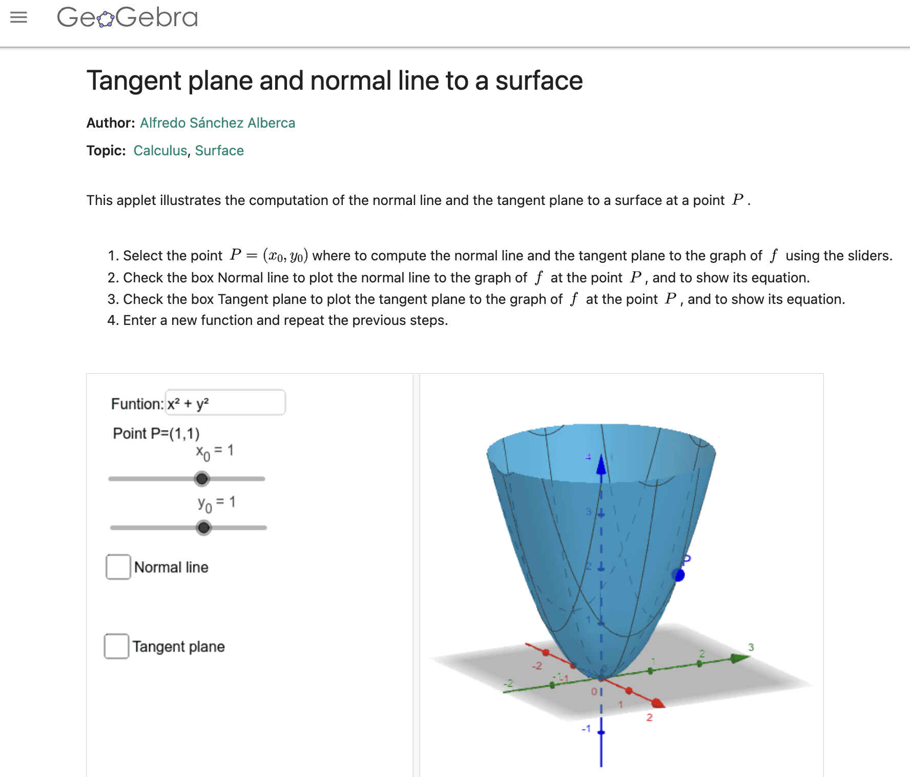
If melons and basketballs are not your style, you can play the same game on an interactive graph of a function with two inputs. The snapshot below is a link to an applet that shows the graph of a function as a blue surface. You can specify a point on the surface by setting the value of the (x, y) input using the sliders. Display the tangent plane (which will be green) at that point by check-marking the “Tangent plane” input. (Acknowledgments to Alfredo Sánchez Alberca who wrote the applet using the GeoGebra math visualization system.)
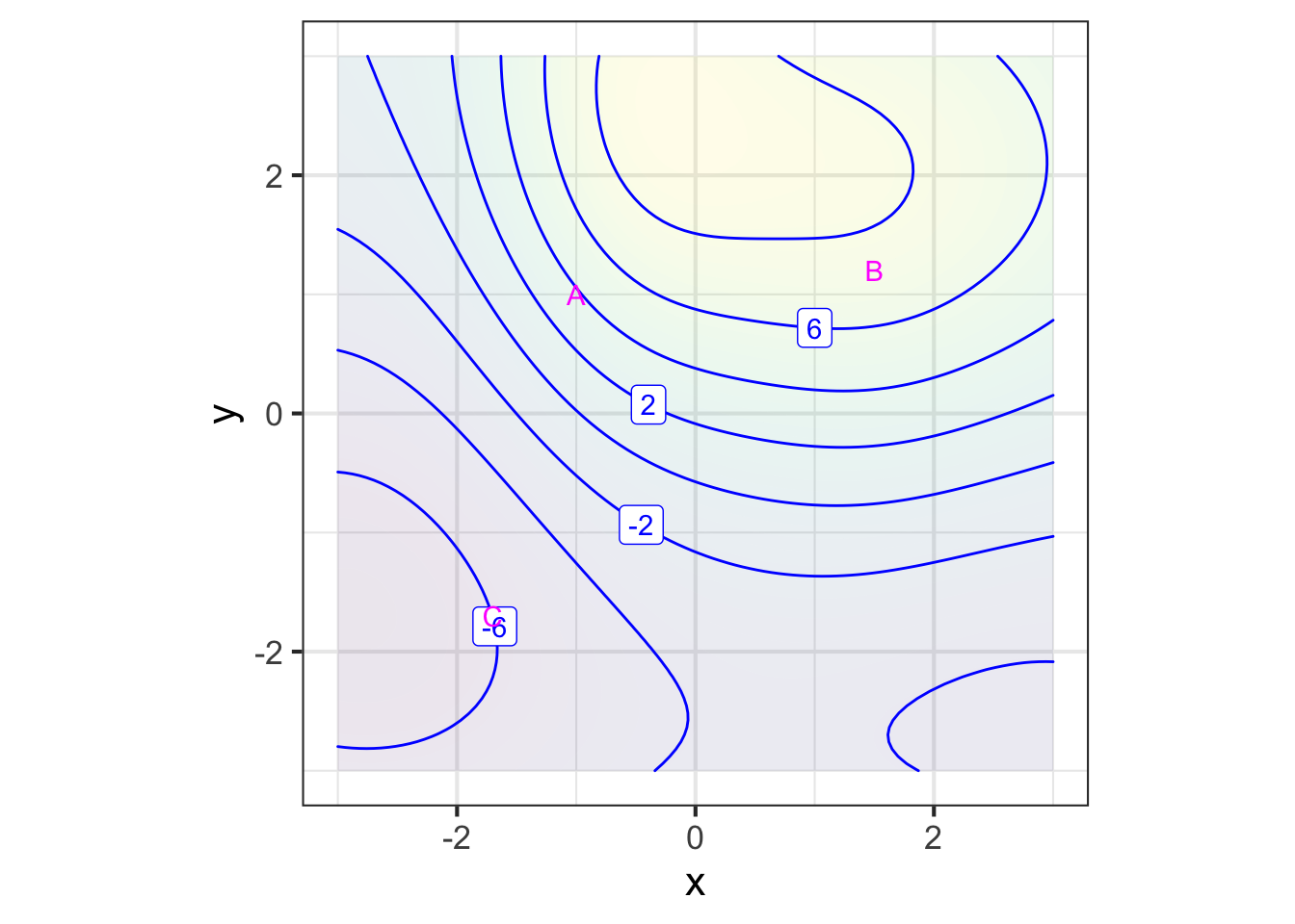
For the purposes of computation by eye, a contour graph of a surface can be easier to deal with. Figure fig-whole-plot shows the contour graph of a smoothly varying function. Three points have been labeled A, B, and C.
Zooming in on each of the marked points presents a simpler picture for each of them, although one that is different for each point. Each zoomed-in plot contains almost parallel, almost evenly spaced contours. If the surface had been exactly planar over the entire zoomed-in domain, the contours would be exactly parallel and exactly evenly spaced. We can approach such exact parallelness by zooming in more closely around the labeled point.
Just as the function \(\line(x) \equiv a x + b\) describes a straight line, the function \(\text{plane}(x, y) \equiv a + b x + c y\) describes a plane whose orientation is specified by the value of the parameters \(b\) and \(c\). (Parameter \(a\) is about the vertical location of the plane, not its orientation.)
The linear approximation shown in each panel of Figure fig-zoomed-plot has the same orientation as the actual function; the contours face in the same way.
Remember that the point of constructing such facets is to generalize the idea of a derivative from a function of one input \(f(x)\) to functions of two or more inputs such as \(g(x,y)\). Just as the derivative \(\partial_x f(x_0)\) reflects the slope of the line tangent to the graph of \(f(x)\) at \(x=x_0\), our plan for the “derivative” of \(g(x_0,y_0)\) is to represent the orientation of the facet tangent to the graph of \(g(x,y)\) at \((x=x_0, y=y_0)\). The question for us now is what information is needed to specify an orientation.
One clue comes from the formula for a function whose graph is a plane oriented in a particular direction:
\[\text{plane}(x,y) \equiv a + b x + cy\]
Try it! try-move-book Plane orientation, analog version
An instructive experience is to pick up a rigid, flat object, for instance a smartphone or hardcover book. Hold the object level with pinched fingers at the mid-point of each of the short ends, as shown in Figure fig-hold-book (left).
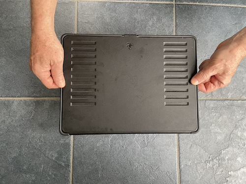
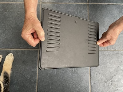
You can tip the object in one direction by raising or lowering one hand. (panel b) You can tip the object in the other coordinate (panel c) by rotating your thumb and forefinger while keeping hand level constant. By combining these two motions, you can orient the surface of the object in a wide range of directions.
Pilots or sailors know that the orientation of an object—a plane or a boat—is described by three parameter: pitch, roll, and yaw. What’s different for a planar facet? It has no front or back end, unlike a plane or boat, so yaw doesn’t apply. Only pitch and roll are needed to describe the orientation of the facet.
The point here is to show that two numbers are sufficient to dictate the orientation of a plane. Referring to Figure fig-hold-book these are 1) the amount that one hand is raised relative to the other and 2) the angle of rotation around the hand-to-hand axis.
Similarly, in the formula for a plane, the orientation is set by two numbers, \(b\) and \(c\) in \(\text{plane}(x, y) \equiv a + b x + c y\).
How do we find the right \(b\) and \(c\) for the tangent facet to a function \(g(x,y)\) at a specific input \((x_0, y_0)\)? Taking slices of \(g(x,y)\) provides the answer. In particular, these two slices: \[\text{slice}_1(x) \equiv g(x, y_0) = a + b\, x + c\, y_0 \\ \text{slice}_2(y) \equiv g(x_0, y) = a + b x_0 + c\, y\]
Look carefully at the formulas for the slices. In \(\text{slice}_1(x)\), the value of \(y\) is being held constant at \(y=y_0\). Similarly, in \(\text{slice}_2(y)\) the value of \(x\) is held constant at \(x=x_0\).
The parameters \(b\) and \(c\) can be read out from the derivatives of the respective slices: \(b\) is equal to the derivative of the slice\(_1\) function with respect to \(x\) evaluated at \(x=x_0\), while \(c\) is the derivative of the slice\(_2\) function with respect to \(y\) evaluated at \(y=y_0\). Or, in the more compact mathematical notation:
\[b = \partial_x \text{slice}_1(x)\left.\strut\right|_{x=x_0} \ \ \text{and}\ \ c=\partial_y \text{slice}_2(y)\left.\strut\right|_{y=y_0}\] These derivatives of slice functions are called partial derivatives. The word “partial” refers to examining just one input at a time. In the above formulas, the \({\large |}_{x=x_0}\) means to evaluate the derivative at \(x=x_0\) and \({\large |}_{y=y_0}\) means something similar.
You need not create the slices explicitly to calculate the partial derivatives. Simply differentiate \(g(x, y)\) with respect to \(x\) to get parameter \(b\) and differentiate \(g(x, y)\) with respect to \(y\) to get parameter \(c\). To demonstrate, we will make use of the sum rule: \[\partial_x g(x, y) = \underbrace{\partial_x a}_{=0} + \underbrace{\partial_x b x}_{=b} + \underbrace{\partial_x cy}_{=0} = b\] Similarly, \[\partial_y g(x, y) = \underbrace{\partial_y a}_{=0} + \underbrace{\partial_y b x}_{=0} + \underbrace{\partial_y cy}_{=c} = c\]
Tip
Get in the habit of noticing the subscript on the differentiation symbol \(\partial\). When taking, for instance, \(\partial_y f(x,y,z, \ldots)\), all inputs other than \(y\) are to be held constant. Some examples:
\[\partial_y 3 x^2 = 0\ \ \text{but}\ \ \ \partial_x 3 x^2 = 6x\\ \ \\ \partial_y 2 x^2 y = 2x^2\ \ \text{but}\ \ \ \partial_x 2 x^2 y = 4 x y \]
25.2 All other things being equal
Recall that the derivative of a function with one input, say, \(\partial_x f(x)\) tells you, at each possible value of the input \(x\), how much the output will change proportional to a small change in the value of the input.
Now that we are in the domain of multiple inputs, writing \(h\) to stand for “a small change” is not entirely adequate. Instead, we will write \(dx\) for a small change in the \(x\) input and \(dy\) for a small change in the \(y\) input.
With this notation, we write the first-order polynomial approximation to a function of a single input \(x\) as \[f(x+dx) = f(x) + \partial_x f(x) \times dx\] Applying this notation to functions of two inputs, we have: \[g(x + {\color{magenta}{dx}}, y) = g(x,y) + {\color{magenta}{\partial_x}} g(x,y) \times {\color{magenta}{dx}}\] and \[g(x, y+{\color{brown}{dy}}) = g(x,y) + {\color{brown}{\partial_y}} g(x,y) \times {\color{brown}{dy}}\]
Each of these statements is about changing one input while holding the other input(s) constant. Or, as the more familiar expression goes, “The effect of changing one input all other things being equal or all other things held constant. (The Latin phrase for this is ceteris paribus, often used in economics.)
Everything we’ve said about differentiation rules applies not just to functions of one input, \(f(x)\), but to functions with two or more inputs, \(g(x,y)\), \(h(x,y,z)\) and so on.
25.3 Gradient vector
For functions of two inputs, there are two partial derivatives. For functions of three inputs, there are three partial derivatives. We can, of course, collect the partial derivatives into Cartesian coordinate form. This collection is called the gradient vector.
Just as our notation for differences (\(\cal D\)) and derivatives (\(\partial\)) involves unusual typography on the letter “D,” the notation for the gradient involves such unusual typography although this time on \(\Delta\), the Greek version of “D.” For the gradient symbol, turn \(\Delta\) on its head: \(\nabla\). That is, \[\nabla g(x,y) \equiv \left(\stackrel\strut\strut\partial_x g(x,y), \ \ \partial_y g(x,y)\right)\]
Note that \(\nabla g(x,y)\) is a function of both \(x\) and \(y\), so in general the gradient vector differs from place to place in the function’s domain.
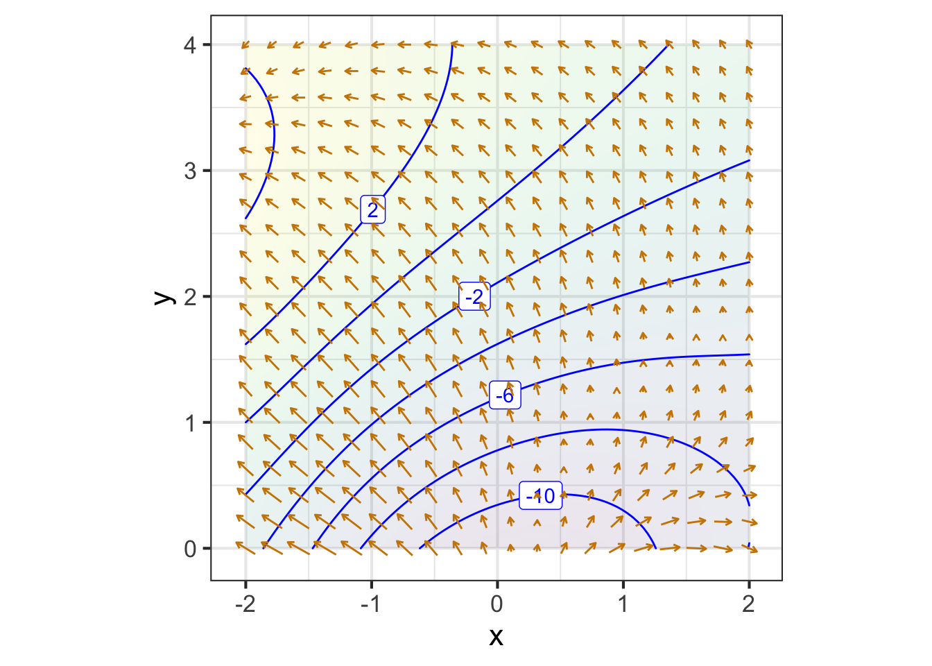
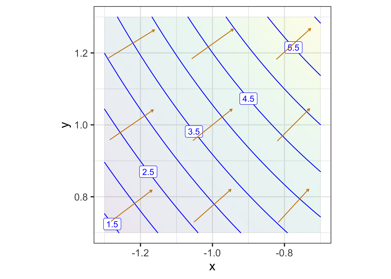
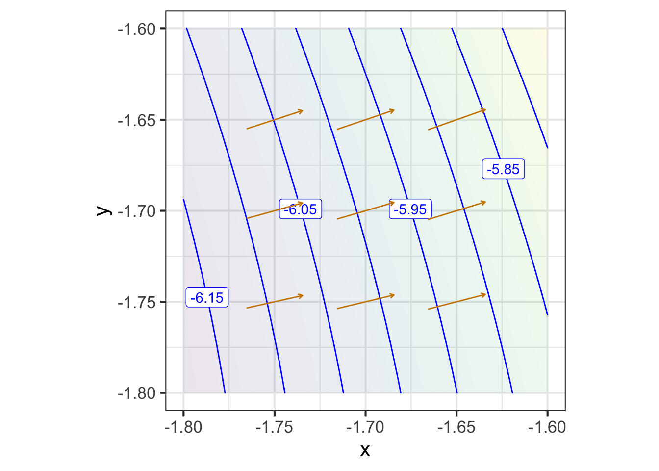
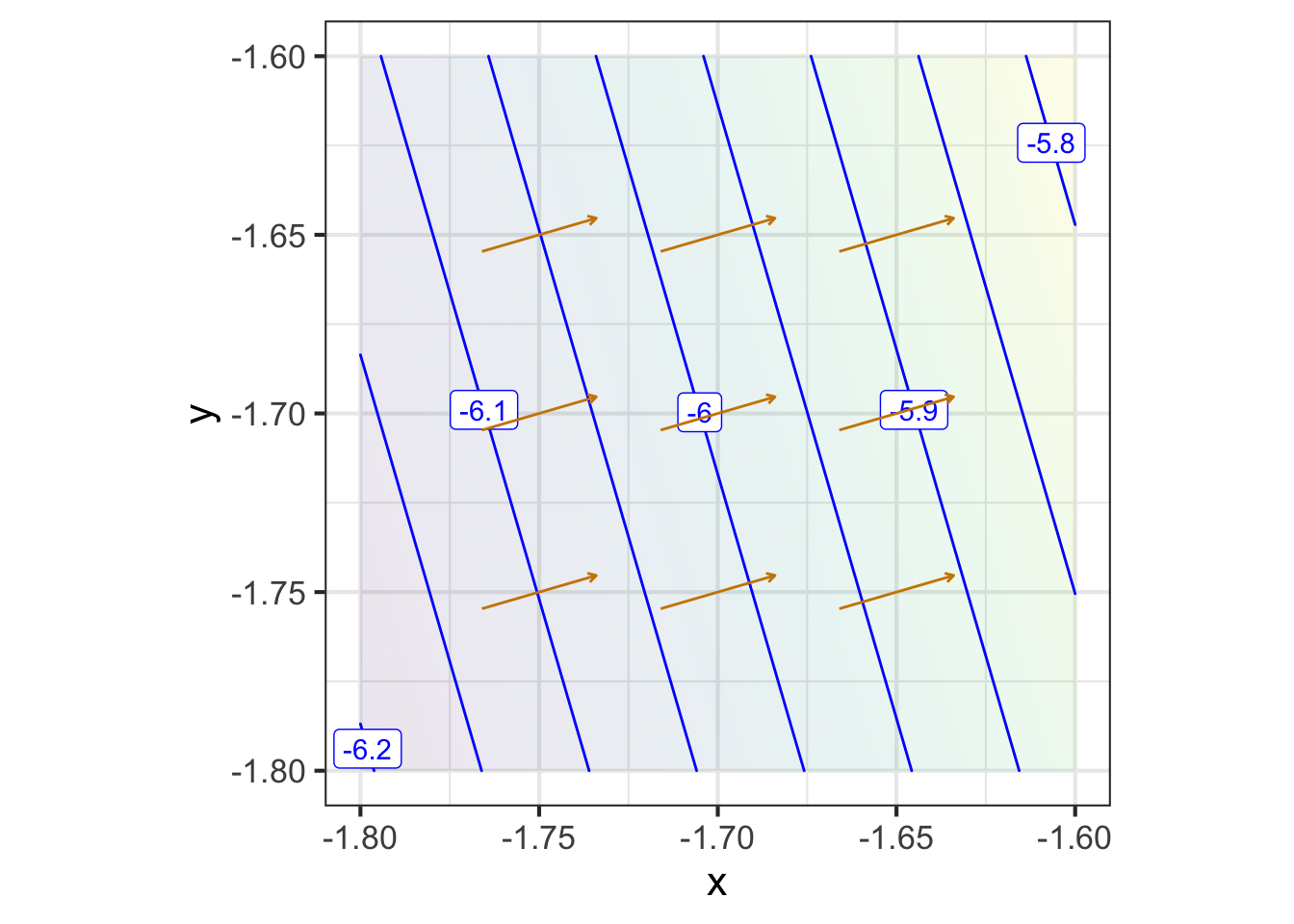
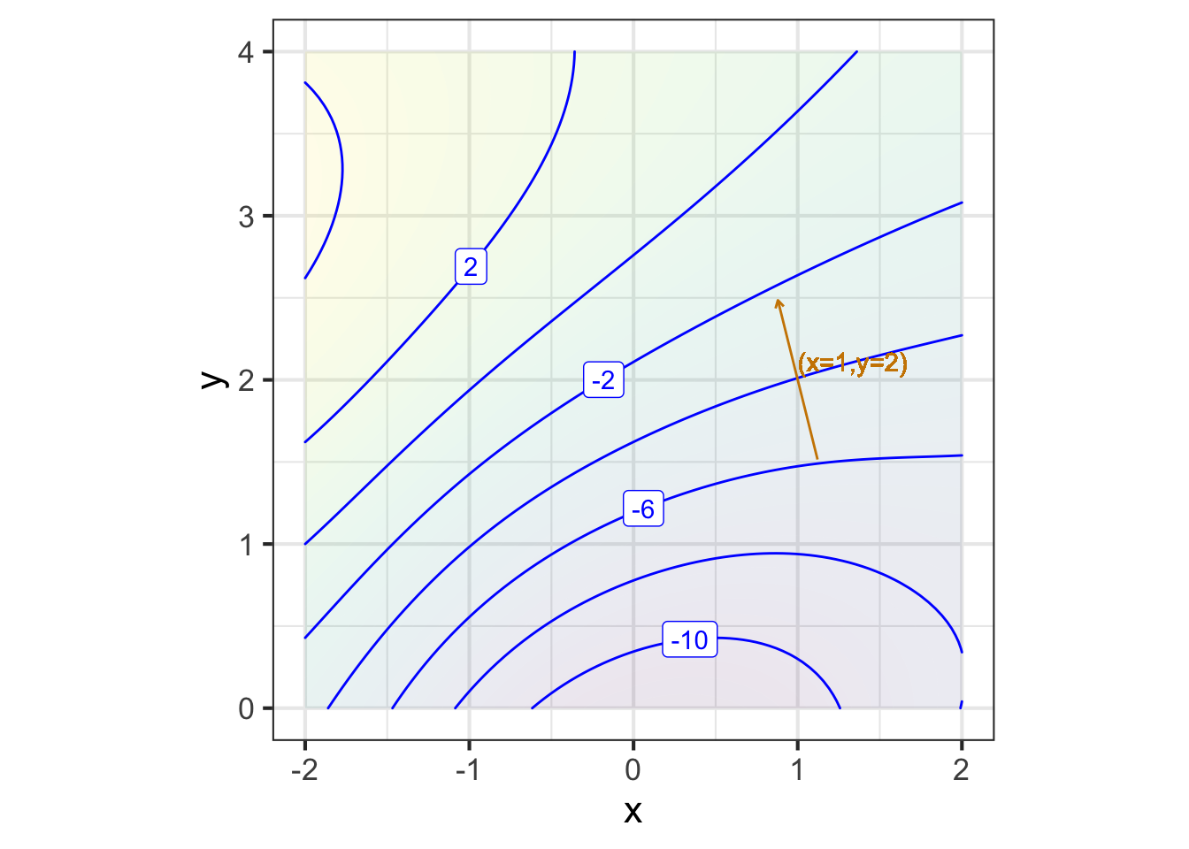
The graphics convention for drawing a gradient vector for a particular input, that is, \(\nabla g(x_0, y_0)\), puts an arrow with its root at \((x_0, y_0)\), pointing in direction \(\nabla g(x_0, y_0)\), as in Figure fig-one-grad-arrow.
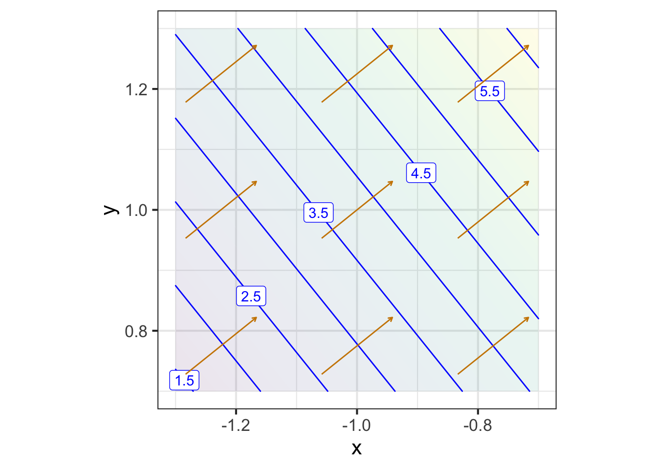
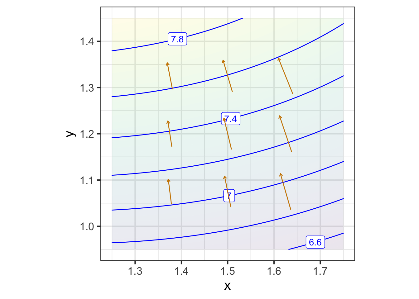
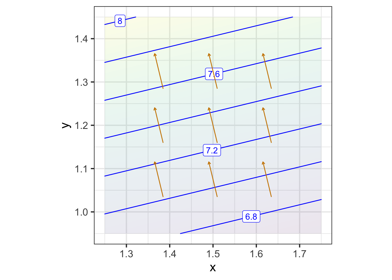
A gradient field (see Figure fig-gradient-field-A) is the value of the gradient vector at each point in the function’s domain. Graphically, to prevent over-crowding, the vectors are drawn at discrete points. The lengths of the drawn vectors are set proportional to the numerical length of \(\nabla g(x, y)\), so a short vector means the surface is relatively level, a long vector means the surface is relatively steep.