27 Polynomials for approximating functions
Almost all readers of this book will have studied mathematics previously. Those who reached secondary school very likely spent considerable time factoring polynomials, sometimes called “finding the roots.” Many students still remember the “quadratic formula” from high school, which will find applications later in this book.
Students and their instructors often struggle to explain what non-textbook problems are solved with factoring polynomials. There are uncountable numbers of posts on the internet addressing the question, many of which refer to the “beauty” of algebra, its benefits in learning logical thinking, and then kick the can down the road by saying that it is crucial to understanding calculus and other mathematical topics at the college level.
You have already seen in sec-low-order how low-order polynomials provide a framework for arranging our intuitive understanding of real-world settings into quick mathematical models of those settings, for instance, in Application area thm-simple-experiments on modeling the speed of a bicycle as a function of steepness of the road and the gear selected for pedaling.
Calculus textbooks have for generations described using polynomials for better theoretical understanding of functions. This author, like many, was so extensively trained in the algebraic use of polynomials that it is practically impossible to ascertain the extent to which they are genuinely useful in developing understanding of the uses of math. It seems wise to follow tradition and include mention of classical textbook problems in this book. That’s one goal of this chapter. But it’s common for polynomials to be used for modeling problems for which they are poorly suited, and even to focus on aspects of functions such as higher-order derivatives, that get in the way of productive work.
27.1 Hundreds of years ago ….
Fifteen-hundred years ago, the Indian mathematician Brahmagupta (c. 598 – c. 668 CE) published what is credited as the first clear statement of the quadratic theorem. Clear perhaps to scholars of ancient mathematics and its unfamiliar notation, but not to the general modern reader.
Brahmagupta’s text also include the earliest known use of zero as a number in its own right, as opposed to being a placeholder in other numbers. He published rules for arithmetic with zero and negative numbers that will be familiar to most (perhaps all) readers of this book. However, his comments on division by zero, for instance that \(\frac{0}{0} = 0\) are not consistent with modern understanding. Today, constructions such as \(\frac{0}{0}\) are called indeterminate forms, even though many beginning students are inclined to prefer Brahmagupta’s opinion on the matter. I mention this because the calculus of indeterminate forms, which resolves many questions previously unresolved since antiquity, are a staple of calculus textbooks.
Much earlier records from Babylonian clay tablets show that mathematicians were factoring quadratics as long ago as 2000-1600 BC.
In the 15th and 16th century CE, mathematicians such as Scipione del Ferro and Niccolò Tartaglia were stars of royal competitions in factoring polynomials. Such competitions were one way for mathematicians to secure support from wealthy patrons. The competitive environment encouraged mathematicians to keep their findings secret, a attitude which was common up until the late 1600s when Enlightenment scholars came to value the sort of open publication which is a defining element of science today. Young Isaac Newton was elected a fellow of the newly founded Royal Society—full name: the Royal Society of London for Improving Natural Knowledge—in 1672 and was president from 1703 until his death a quarter century later.
This is a long and proud history for polynomials, perhaps in itself justifying their placement near the center of the high-school curriculum. It’s easy to see the strong motivation mathematicians would have in the early years of calculus to apply their new tools to understanding polynomials and, later, functions. The importance of polynomials to mathematical culture is signaled by the distinguished name given to the proof that an nth-order polynomial has exactly n roots: the Fundamental theorem of algebra.
As for factoring polynomials, in the 1500s mathematicians found formulas for roots of third- and fourth-order polynomials. Today, they are mainly historical artifacts since the arithmetic involved is subject to catastrophic round-off error. By 1824, the formulas-for-factoring road came to a dead end when it was proved that fifth- and higher-order polynomials do not have general solutions written only using square roots or other radicals.
27.2 A warning for modelers
Later in this chapter, we’ll return to address classical mathematical problems using polynomials. This section is about the pitfalls of using third- and higher-order polynomials in constructing models of real-world settings. (As mentioned previously, low-order polynomials are a different matter. See sec-low-order.)
Building a reliable model with high-order polynomials requires a deep knowledge of mathematics and introduces serious potential pitfalls. Modern professional modelers learn the alternatives to high-order polynomials (for example, “natural splines” and “radial basis functions”), but newcomers often draw on their high school experience and give unwarranted credence to polynomials.
The domain of polynomials, like the power-law functions they are assembled from, is the real numbers, that is, the entire number line \(-\infty < x < \infty\). (More precisely, the domain is the complex numbers, of which the real numbers are an infinitesimal subset. We’ll look at modeling uses for complex numbers in sec-second-order-de.)
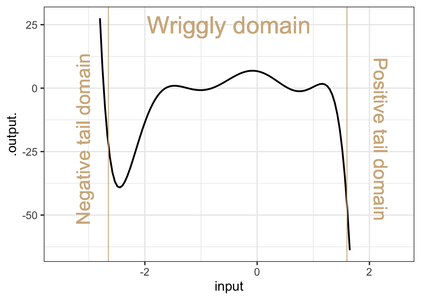
To understand the shape of high-order polynomials, it is helpful to divide the domain into three parts: a wiggly domain at the center and two tail domains, one on the right side and the other on the left.
Figure fig-wriggly-polynomial shows a 7th order polynomial—that is, the highest-order term is \(x^7\). In the wriggly domain in Figure fig-wriggly-polynomial, there are six argmins or argmaxes. In one of the tail domains the function value heads off to \(\infty\), in the other to \(-\infty\). This is an inescapable feature of all odd-order polynomials: 1, 3, 5, 7, …
In contrast, for even-order polynomials (2, 4, 6, …) the function values in the two tail domains go in the same direction, either to \(\infty\) (Hands up!) or to \(-\infty\).
Polynomials’ runaway behavior does not provide insurance against wild, misleading extrapolations of model formulas. Instead, sigmoid, Gaussian, and sinusoid functions, as well as more modern constructions such as “smoothers,” “natural splines,” and the “wavelets” originating in fractal theory, provide such insurance.
27.3 Indeterminate forms
Let’s return to an issue that has bedeviled mathematicians for millennia and misled even the famous Brahmagupta. This is the question of dividing zero by zero or, more generally, dividing any number by zero.
Elementary-school students learn that it is illegal to “divide by zero.” Happily, the punishment for breaking the law is, for most students, a deep red mark on a homework or exam paper. Much more serious consequences, however, can sometimes occur, especially in computer programming. (See sec-computing-indeterminate.)
There is a legal loophole, however, that arises in functions like \[\text{sinc}(x) \equiv \frac{\sin(x)}{x}\] that involve an input in a position to cause a division by zero, as with the denominator in \(\frac{\sin(x)}{x}\).
The sinc() function (pronounced “sink”) is important today, in part because of its role in converting discrete-time measurements (as in an mp3 recording of sound into continuous signals. So there really are occasions that call for evaluating it at zero input.
What is the value of \(\text{sinc}(0)\)? One answer, favored by arithmetic teachers is that \(\text{sinc}(0)\) is meaningless, because it involves division by zero.
On the other hand, \(\sin(0) = 0\) as well, so the sinc function evaluated at zero involves 0/0. This quotient is called an indeterminate form. The logic is this: Suppose \(0/0 = b\) for some number \(b\). then \(0 = 0 \times b = 0\). So any value of \(b\) would do; the value of \(0/0\) is “indeterminate.”
Still another answer is suggested by plotting out sinc(\(x\)) near \(x=0\) and reading the value off the graph: sinc(0) = 1.
To judge from the output of Active R chunk lst-sinc-near-zero, \(\sin(0) / 0 = 1\).
The graph of sinc() looks smooth and the shape makes sense. Even if we zoom in very close to \(x=0\), the graph continues to look smooth. We call such functions well behaved.
Compare the well-behaved sinc() to a very closely related function (which does not seem to be so important in applied work): \(\frac{\sin(x)}{x^3}\).
Both \(\sin(x)/x\) and \(\sin(x) / x^3\) involve a divide by zero when evaluated at \(x=0\). Both are indeterminate forms 0/0 at \(x=0\). But the graph of \(\sin(x) / x^3\) (see Active R chunk lst-sinc2) is not well behaved. \(\sin(x) / x^3\) does not have any particular value at \(x=0\); instead, it has an asymptote.
Active R chunk lst-sinc2 zooms in around the division by zero. Top: The graph of \(\sin(x)/x\) versus \(x\). Bottom: The graph of \(\sin(x)/x^2\). The vertical scales on the two graphs are utterly different.
Since both \(\sin(x)/x\left.{\Large\strut}\right|_{x=0}\) and \(\sin(x)/x^3\left. {\Large\strut}\right|_{x=0}\) involve a divide-by-zero, the answer to the utterly different behavior of the two functions is not to be found at zero. Instead, it is to be found near zero. For any non-zero value of \(x\), the arithmetic to evaluate the functions is straight-forward. Note that \(\sin(x) / x^3\) starts its mis-behavior away from zero. The slope of \(\sin(x) / x^3\) is very large near \(x=0\), while the slope of \(\sin(x) / x\) smoothly approaches zero.
Since we are interested in behavior near \(x=0\), a useful technique is to approximate the numerator and denominator of both functions by polynomial approximations.
- \(\sin(x) \approx x - \frac{1}{6} x^3\) near \(x=0\)
- \(x\) is already a polynomial.
- \(x^3\) is already a polynomial.
As we will see in sec-high-order-approx , these approximations are exact as \(x\) goes to zero. So, when \(x\) is sufficiently small, that is, evanescent,
\[\frac{\sin(x)}{x} = \frac{x - \frac{1}{6} x^3}{x} = 1 + \frac{1}{6} x^2\] Even at \(x=0\), there is nothing indeterminate about \(1 + x^2/6\); it is simply 1.
Compare this to the polynomial approximation to \(\sin(x) / x^3\): \[\frac{\sin(x)}{x^3} = \frac{x - \frac{1}{6} x^3}{x^3} = \frac{1}{x^2} - \frac{1}{6}\]
Evaluating this at \(x=0\) involves division by zero. No wonder it is badly behaved.
The procedure for checking whether a function involving division by zero behaves well or poorly is described in the first-ever calculus textbook, published in 1697. The title (in English) is: The analysis into the infinitely small for the understanding of curved lines. In honor of the author, the Marquis de l’Hospital, the procedure is called l’Hôpital’s rule.1
Conventionally, the relationship is written \[\lim_{x\rightarrow x_0} \frac{u(x)}{v(x)} = \lim_{x\rightarrow x_0} \frac{\partial_x u(x)}{\partial_x v(x)}\]
Let’s try this out with our two example functions around \(x=0\):
\[\lim_{x\rightarrow 0} \frac{\sin(x)}{x} = \frac{\lim_{x\rightarrow 0} \cos(x)}{\lim_{x \rightarrow 0} 1} = \frac{1}{1} = 1\]
\[\lim_{x\rightarrow 0} \frac{\sin(x)}{x^3} = \frac{\lim_{x\rightarrow 0} \cos(x)}{\lim_{x \rightarrow 0} 3x^2} = \frac{1}{0} \ \ \ \ \text{Indeterminate}!\] There are other indeterminate forms that involve infinity rather than zero. The mathematical symbol for infinity, \(\infty\), was introduced for this purpose in 1655 but the character has a much longer history as a decorative item. The key to understanding indeterminate forms involving \(\infty\) is to recognize that it is closely related to \(\frac{1}{0}\).
A careless author who states simply that \(\infty \equiv \frac{1}{0}\) will earn the contempt of mathematicians who understand that legitimate statements can only be made when they involve the evanescent, as in \[\lim_{h \rightarrow 0} \frac{1}{h}\] which states clearly that \(h \neq 0\).But using the sloppy, non-evanescent notation is convenient for starting to understand why constructions like \[\infty \times 0\ \ \text{or}\ \ \frac{\infty}{\infty}\] are indeterminate forms related to \(\frac{0}{0}\). Using the sloppy notation \(\infty \equiv \frac{1}{0}\) provides clarity:
\[\infty \times 0 = \frac{1}{0} \times 0 = \frac{1 \times 0}{0} = \frac{0}{0}\ \ \text{and, similarly, }\ \ \frac{\infty}{\infty} = \frac{1/0}{1/0} = 0/0 .\]
27.4 Computing with indeterminate forms
In the early days of electronic computers, division by zero would cause a fault in the computer, often signaled by stopping the calculation and printing an error message to some display. This was inconvenient since programmers did not always foresee and avoid division-by-zero situations.
As you’ve seen, modern computers have adopted a convention that simplifies programming considerably. Instead of stopping the calculation, the computer just carries on normally, but produces as a result one of two indeterminate forms: Inf and NaN.
Inf is the output for the simple case of dividing zero into a non-zero number, for instance:
NaN, standing for “not a number,” is the output for more challenging cases: dividing zero into zero, multiplying Inf by zero, or dividing Inf by Inf.
The idea’s brilliance is that any calculation that involves NaN will return a value of NaN. This might seem to get us nowhere. However, most programs are built out of other programs, usually written by people interested in different applications. You can use those programs (mostly) without worrying about the implications of a divide by zero. If it is important to respond in some particular way, you can always check the result for being NaN in your own programs. (Much the same is true for Inf, although dividing a non-Inf number by Inf will return 0.)
Plotting software will often treat NaN values as “don’t plot this.” that is why it is possible to make a sensible plot of \(\sin(x)/x\) even when the plotting domain includes zero.
27.5 Multiple inputs?
High-order polynomials are rarely used with multiple inputs. One reason is the proliferation of coefficients. For instance, here is the third-order polynomial in two inputs, \(x\), and \(y\). \[\underbrace{b_0 + b_x x + b_y y}_\text{first-order terms} + \underbrace{b_{xy} x y + b_{xx} x^2 + b_{yy} y^2}_\text{second-order terms} + \underbrace{b_{xxy} x^2 y + b_{xyy} x y^2 + b_{xxx} x^3 + b_{yyy} y^3}_\text{third-order terms}\]
This has 10 coefficients. With so many coefficients it is hard to ascribe meaning to any of them individually. And, insofar as some feature of the function does carry meaning in the modeling situation, that meaning is spread out and hard to quantify.
27.6 High-order approximations
Despite the pitfalls of high-order polynomials, they are dear to theoretical mathematicians. In particular, mathematicians find benefits to approximating known functions by high-order polynomials.
The applied student might wonder, what is the point of approximating known functions. If we know the function, why approximate? One good reason is to simplify calculations. For instance, suppose you need the value of the pattern-book function \(\ln(x)\) near \(x=1\). We know a lot about \(\ln(x)\) at \(x=1\) which we can use to construct a simple approximation for the nearby values. For instance, in sec-pattern-book-functions we emphasized the fact that \(\ln(1) = 0\).
Another important fact about \(\ln(x)\) at zero is its derivative \(\partial_x \ln(x)\). Using the differentiation rules from sec-prod-comp-rules we can perform a useful trick. We know that the exponential function and logarithmic functions are inverses, that is,
\[\ln(\exp(x)) = x . \tag{27.1}\]
Let’s differentiate both sides. The right-hand side is easy: \(\partial_x x = 1\). The left-hand side is a bit more intricate. Using the chain rule on the left gives
\[\partial_x \ln(\exp(x)) = \partial_x \ln (\exp(x)) \times \partial_x \exp(x) = \exp(x) \times \partial_x \ln(\exp(x))\] which may not look like a promising start. But, remembering that the derivative of the right-hand side of #eq-log-exp-x is 1, we have:
\[\partial_x \ln(\exp(x)) = \frac{1}{\exp(x)}\] Whatever the input \(x\) is, the output of \(\exp(x)\) is some number. Let’s call that number \(y\). This gives \[\partial_x \ln(y) = \frac{1}{y}.\] At \(y=1\), \(\partial_y\ln(1) = 1\). But \(y\) is just the name of the argument and we can replace that name with any other, for instance, \(x\). So \(\partial_x\ln(x=1) = 1.\)
It’s easy to differentiate power-law functions like \(1/x\). For instance: \[\partial_x \frac{1}{x} = - \frac{1}{x^2} \ \ \text{and}\ \ \partial_{xx} \frac{1}{x} = - \partial_x \left[\frac{1}{x^2}\right] = \frac{2}{x^3} .\] We can keep on going in this manner to find higher derivatives, all of which will have a form like \(\pm \frac{(n-1)!}{x^n}\). Evaluated at \(x=1\), our input of interest, these become \(\pm (n-1)!\) for the nth derivative.
In other words, we know a lot about \(\ln(x)\) at \(x=1\)—the function value as well as all of its derivatives.
For polynomials, the output can be calculated using just multiplication and addition, which makes them attractive for numerical evaluation. As well we can differentiate to any order any polynomial. And, with a bit of practice, we can write down a polynomial whose derivative is a given number at some input value. Once we have learned how to do this, we can, for instance, write down a polynomial that shares the value and derivatives of \(\ln(x)\) at \(x=1\). Such a polynomial is called a Taylor Polynomial. If we imagine writing down such a polynomial to infinite order, the result is called a Taylor Series.
The significance of this fact is that we can write a polynomial approximation to any function whose value and derivatives can be evaluated, if only at a single input value like \(x=1\) we used for \(\ln(x)\).
To illustrate, consider another pattern-book function, \(\sin(x)\). We know the value of \(\sin(x=0) = 0\). We can also calculate the derivatives of any order; just walk down the sequence \[\cos(x), -\sin(x), - \cos(x), \sin(x), ...\] and so on in a repeating cycle. Thus, we know the numerical value of \(\sin()\) and its derivatives of any order at an input \(x=0\), using the fact that \(\cos(0) = 1\).
Consider this polynomial: \[g(x) \equiv x - \frac{1}{6} x^3\] Since the highest-order term is \(x^3\) this is a third-order polynomial. (As you will see, we picked these particular coefficients, 0, 1, 0, -1/6, for a reason.) With such simple coefficients the polynomial is easy to handle by mental arithmetic. For instance, for \(g(x=1)\) is \(5/6\). Similarly, \(g(x=1/2) = 23/48\) and \(g(x=2) = 2/3\). A person of today’s generation would use an electronic calculator for more complicated inputs, but the mathematicians of Newton’s time were accomplished human calculators. It would have been well within their capabilities to calculate, using paper and pencil, \(g(\pi/4) = 0.7046527\).2
Our example polynomial, \(g(x) \equiv x - \frac{1}{6}x^3\), graphed in color in Figure fig-small-sine, does not look exactly like the sinusoid. If we increased the extent of the graphics domain, the disagreement would be even more striking, since the sinusoid’s output is always in \(-1 \leq \sin(x) \leq 1\), while the polynomial’s tails are heading off to \(\infty\) and \(-\infty\). But, for a small interval around \(x=0\), exactly aligns with the sinusoid.
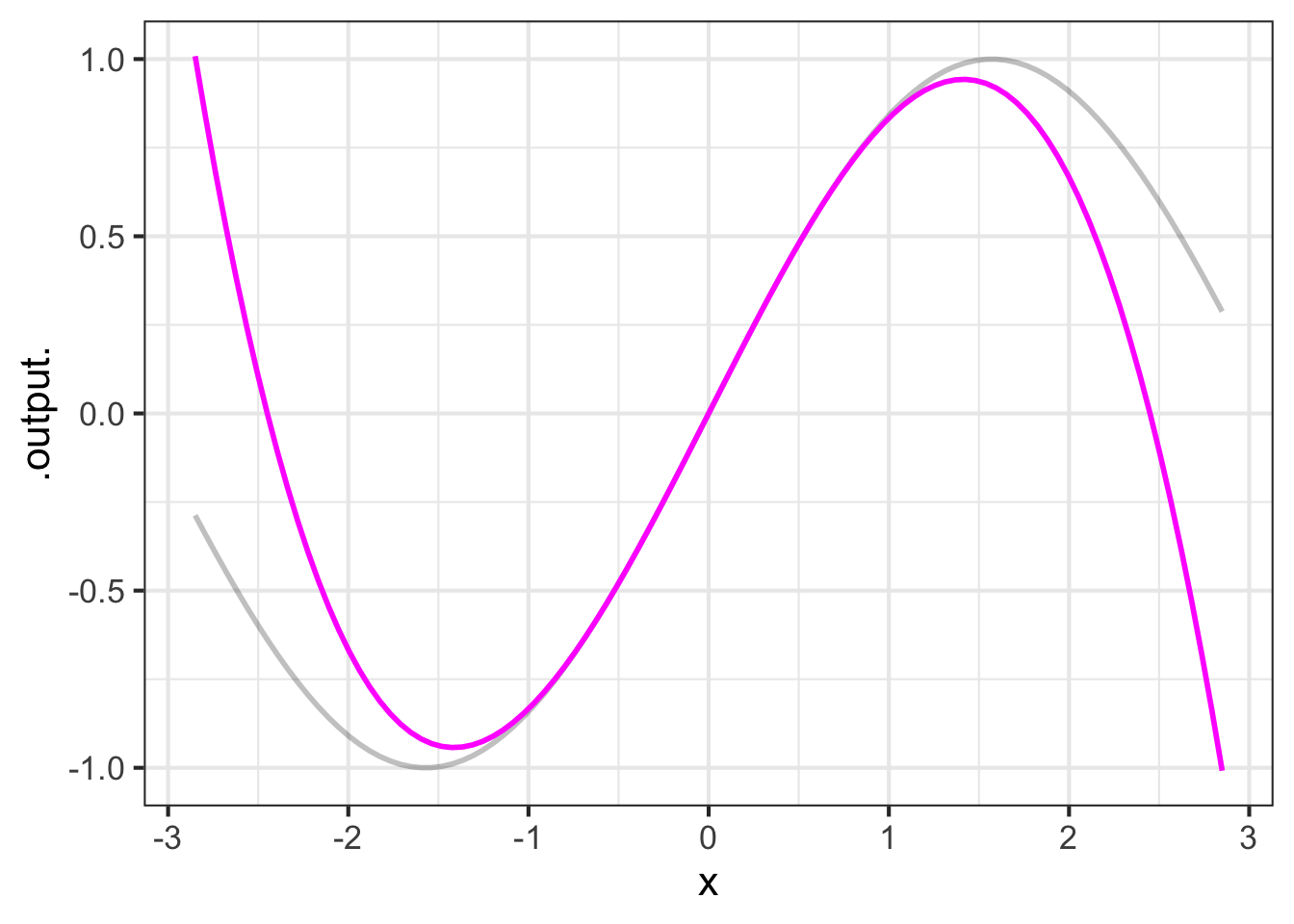
It is clear from the graph that the approximation is excellent near \(x=0\) and gets worse as \(x\) gets larger. The approximation is poor for \(x \approx \pm 2\). We know enough about polynomials to say that the approximation will not get better for larger \(x\); the sine function has a range of \(-1\) to \(1\), while the left and right tails of the polynomial are running off to \(\infty\) and \(-\infty\) respectively.
One way to measure the quality of the approximation is the error \({\cal E}(x)\) which gives, as a function of \(x\), the difference between the actual sinusoid and the approximation: \[{\cal E}(x) \equiv |\strut\sin(x) - g(x)|\] The absolute value used in defining the error reflects our interest in how far the approximation is from the actual function and not so much in whether the approximation is below or above the actual function. Figure fig-sin-error shows \({\cal E}(x)\) as a function of \(x\). Since the error is the same on both sides of \(x=0\), only the positive \(x\) domain is shown.
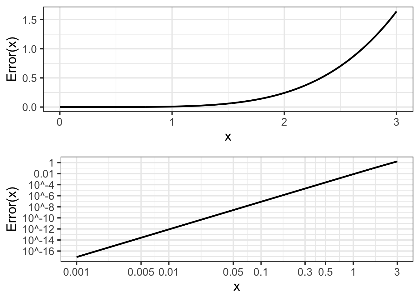
Figure fig-sin-error shows that for \(x < 0.3\), the error in the polynomial approximation to \(\sin(x)\) is in the 5th decimal place. For instance, \(\sin(0.3) = 0.2955202\) while \(g(0.3) = 0.2955000\).
That the graph of \({\cal E}(x)\) is a straight-line on log-log scales diagnoses \({\cal E}(x)\) as a power law. That is: \({\cal E}(x) = A x^p\). As always for power-law functions, we can estimate the exponent \(p\) from the slope of the graph. It is easy to see that the slope is positive, so \(p\) must also be positive.
The inevitable consequence of \({\cal E}(x)\) being a power-law function with positive \(p\) is that \(\lim_{x\rightarrow 0} {\cal E}(x) = 0\). That is, the polynomial approximation \(x - \frac{1}{6}x^3\) is exact as \(x \rightarrow 0\).
Throughout this book, we’ve been using straight-line approximations to functions around an input \(x_0\). \[g(x) = f(x_0) + \partial_x f(x_0) [x-x_0]\] One way to look at \(g(x)\) is as a straight-line function. Another way is as a first-order polynomial. This raises the question of what a second-order polynomial approximation should be. Rather than the polynomial matching just the slope of \(f(x)\) at \(x_0\), we can arrange things so that the second-order polynomial will also match the curvature of the \(f()\). Since the curvature involves only the first and second derivatives of a function, the polynomial constructed to match both the first and the second derivative will necessarily match the slope and curvature of \(f()\). This can be accomplished by setting the polynomial coefficients appropriately.
Start with a general, second-order polynomial centered around \(x_0\): \[g(x) \equiv a_0 + a_1 [x-x_0] + a_2 [x - x_0]^2\] The first- and second-derivatives, evaluated at \(x=x_0\) are: \[\partial_x g(x)\left.{\Large\strut}\right|_{x=x_0} = a_1 + 2 a_2 [x - x_0] \left.{\Large\strut}\right|_{x=x_0} = a_1\] \[\partial_{xx} g(x)\left.{\Large\strut}\right|_{x=x_0} = 2 a_2\] Notice the 2 in the above expression. When we want to express the coefficient \(a_2\) using the second derivative of \(g()\), we will end up with
\[a_2 = \frac{1}{2} \partial_{xx} g(x)\left.{\Large\strut}\right|_{x=x_0}\]
To make \(g(x)\) approximate \(f(x)\) at \(x=x_0\), we need merely set \[a_1 = \partial_x f(x)\left.{\Large\strut}\right|_{x=x_0}\] and \[a_2 = \frac{1}{2} \partial_{xx} f(x) \left.{\Large\strut}\right|_{x=x_0}\] This logic can also be applied to higher-order polynomials. For instance, to match the third derivative of \(f(x)\) at \(x_0\), set \[a_3 = \frac{1}{6} \partial_{xxx} f(x) \left.{\Large\strut}\right|_{x=x_0}\] Remarkably, each coefficient in the approximating polynomial involves only the corresponding order of derivative. \(a_1\) involves only \(\partial_x f(x) \left.{\Large\strut}\right|_{x=x_0}\); the \(a_2\) coefficient involves only \(\partial_{xx} f(x) \left.{\Large\strut}\right|_{x=x_0}\); the \(a_3\) coefficient involves only \(\partial_{xx} f(x) \left.{\Large\strut}\right|_{x=x_0}\), and so on.
Now we can explain where the polynomial that started this section, \(x - \frac{1}{6} x^3\) came from and why those coefficients make the polynmomial approximate the sinusoid near \(x=0\).
| Order | \(\sin(x)\) derivative | \(x - \frac{1}{6}x^3\) derivative |
|---|---|---|
| 0 | \(\sin(x) \left.{\Large\strut}\right|_{x=0} = 0\) | \(\left( 1 - \frac{1}{6}x^3\right)\left.{\Large\strut}\right|_{x=0} = 0\) |
| 1 | \(\cos(x) \left.{\Large\strut}\right|_{x=0} = 1\) | \(\left(1 - \frac{3}{6} x^2\right) \left.{\Large\strut}\right|_{x=0}= 1\) |
| 2 | \(-\sin(x) \left.{\Large\strut}\right|_{x=0} = 0\) | \(\left(- \frac{6}{6} x\right) \left.{\Large\strut}\right|_{x=0} = 0\) |
| 3 | \(-\cos(x) \left.{\Large\strut}\right|_{x=0} = -1\) | \(- 1\left.{\Large\strut}\right|_{x=0} = -1\) |
| 4 | \(\sin(x) \left.{\Large\strut}\right|_{x=0} = 0\) | \(0\left.{\Large\strut}\right|_{x=0} = 0\) |
The first four derivatives of \(x - \frac{1}{6} x^3\) exactly match, at \(x=0\), the first four derivatives of \(\sin(x)\).
The polynomial constructed by matching successive derivatives of a function \(f(x)\) at some input \(x_0\) is called a Taylor polynomial.
Tip 27.1: Practice: a Taylor polynomial for \(e^x\).
Let’s construct a 3rd-order Taylor polynomial approximation to \(f(x) = e^x\) around \(x=0\).
We know it will be a 3rd order polynomial: \[g_{\exp}(x) \equiv a_0 + a_1 x + a_2 x^2 + a_3 x^3\] The exponential function is particularly nice for examples because the function value and all its derivatives are identical: \(e^x\). So
\[f(x= 0) = 1\]
\[ \partial_x f(x=0) = 1\] \[\partial_{xx} f(x=0) = 1\] \[\partial_{xxx} f(x=0) = 1\] and so on.
The function value and derivatives of \(g_{\exp}(x)\) at \(x=0\) are: \[g_{\exp}(x=0) = a_0\] \[\partial_{x}g_{\exp}(x=0) = a_1\] \[\partial_{xx}g_{\exp}(x=0) = 2 a_2\]
\[\partial_{xxx}g_{\exp}(x=0) = 2\cdot3\cdot a_3 = 6\, a_3\] Matching these to the exponential evaluated at \(x=0\), we get \[a_0 = 1\] \[a_1 = 1\] \[a_2 = \frac{1}{2}\] \[a_3 = \frac{1}{2 \cdot 3} = \frac{1}{6}\]
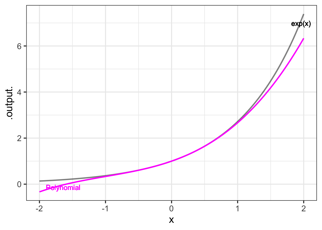
Result: the 3rd-order Taylor polynomial approximation to the exponential at \(x=0\) is \[g_{\exp}(x) = 1 + x + \frac{1}{2} x^2 + \frac{1}{2\cdot 3} x^3 +\frac{1}{2\cdot 3\cdot 4} x^4\]
Figure fig-taylor-exp-3 shows the exponential function \(e^x\) and its 3th-order Taylor polynomial approximation near \(x=0\):

The polynomial is exact at \(x=0\). The error \({\cal E}(x)\) grows with increasing distance from \(x=0\):
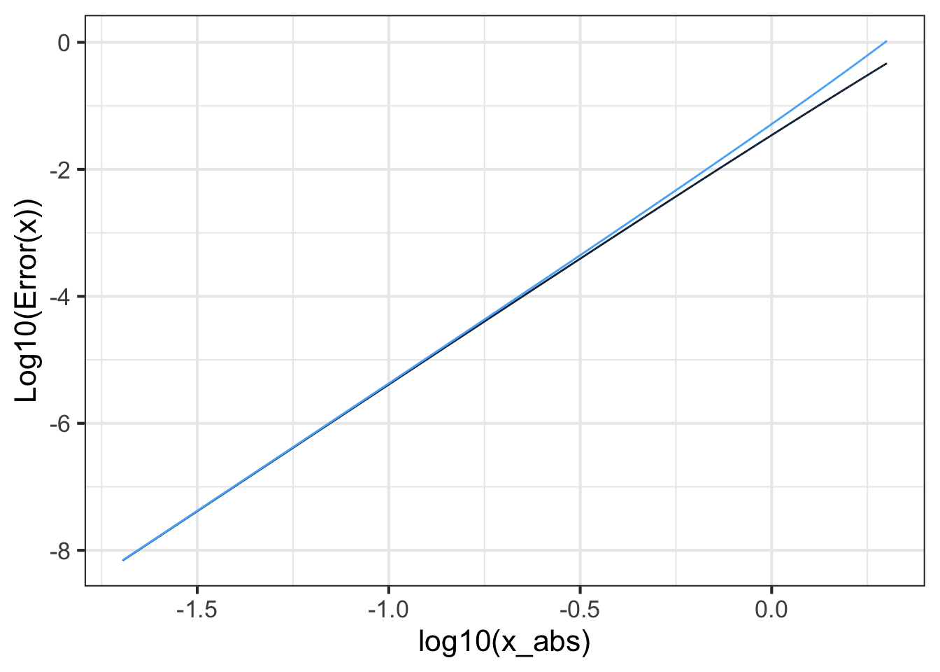
The plot of \(\log_{10} {\cal E}(x)\) versus \(\log_{10} | x |\) in Figure fig-taylor-exp-5 shows that the error grows from zero at \(x=0\) as a power-law function. Measuring the exponent of the power-law from the slope of the graph on log-log axes give \({\cal E}(x) = a |x-x_0|^5\). This is typical of Taylor polynomials: for a polynomial of degree \(n\), the error will grow as a power-law with exponent \(n+1\). This means that the higher is \(n\), the faster \(\lim_{x\rightarrow x_0}{\cal E}(x) \rightarrow 0\). On the other hand, since \({\cal E}_x\) is a power law function, as \(x\) gets further from \(x_0\) the error grows as \(\left(x-x_0\right)^{n+1}\).
Calculus history—Polynomial models of other functions
Brooke Taylor (1685-1731), a near contemporary of Newton, published his work on approximating polynomials in 1715. Wikipedia reports: “[T]he importance of [this] remained unrecognized until 1772, when Joseph-Louis Lagrange realized its usefulness and termed it ‘the main [theoretical] foundation of differential calculus’.”Source

Due to the importance of Taylor polynomials in the development of calculus, and their prominence in many calculus textbooks, many students assume their use extends to constructing models from data. They also assume that third- and higher-order monomials are a good basis for modeling data. Both these assumptions are wrong. Least squares is the proper foundation for working with data.
Taylor’s work preceded by about a century the development of techniques for working with data. One of the pioneers in these new techniques was Carl Friedrich Gauss (1777-1855), after whom the gaussian function is named. Gauss’s techniques are the foundation of an incredibly important statistical method that is ubiquitous today: least squares. Least squares provides an entirely different way to find the coefficients on approximating polynomials (and an infinite variety of other function forms). The R/mosaic fitModel() function for polishing parameter estimates is based on least squares. In Block 5, we will explore least squares and the mathematics underlying the calculations of least-squares estimates of parameters.