23  Derivatives of assembled functions

Chapter 19 used the rules associated with evanescent $h$, that is, $\underset{h\to 0}{lim}$, to confirm our claims about the derivatives of many of the pattern-book functions. We will call these rules h-theory for short. This chapter will use h-theory to find algebraic rules to calculate the derivatives of linear combinations of functions, products of functions, and composition of functions. Remarkably, we can figure out these rules without specifying which functions are being combined. So the rules can be written abstractly using the pronouns $f()$ and $g()$. Later, we will apply those rules to specific functions, to show how the rules are used in practical work.

23.1 Derivatives of the basic modeling functions

Opinions vary about whether it is really worthwhile for students to do extensive problem sets involving differentiating arbitrarily complex functions. But to become conversant with calculus, it helps to know at a glance the derivatives of a few, widely used functions. Section 19.3 introduced symbolic derivatives of each of the pattern-book functions. In general, the pattern-book functions have derivatives that are themselves either pattern-book functions or slight modifications of them. For instance, ${\partial }_x\text{pnorm}(x)\equiv \text{dnorm}(x)$ and ${\partial }_x\ln (x)=\text{recip}(x)$. Most simply of all, ${\partial }_x{e}^x=e^x$.

The basic modeling functions are the same as the pattern-book functions, but with bare $x$ replaced by $\text{line}(x)$. In other words, each of the basic modeling functions is a composition of the corresponding pattern-book function with $\text{line}(x)$. The derivatives of the basic modeling functions are simple variations on the derivatives of the pattern-book functions. It’s easy to learn the rules and well worthwhile committing them to memory.

The “chain rule” provides the underlying logic but takes an especially easy form for the pattern-book functions. We can wait until Section 23.5 to take on the chain rule in general. In the meanwhile, examples will suffice to see how the chain rule plays out in the basic modeling functions.

An example of a basic modeling function is $g(x)\equiv f(ax+b)$ where $f()$ is one of the pattern-book functions. Naturally, we could have used any input name, for instance $g(z)\equiv f(az+b)$ but in the following we will stick to $x$. And while sometimes we write $\text{line}(x)$ as $ax+b$, othertimes we will write an equivalent form: $a(x-x_0)$ or even $\frac{2\pi }{P}(x-x_0)$.

We wish to find the derivative of the basic modeling function with respect to its argument, that is, ${\partial }_{x}g(x)$. The answer is simple:

$$\begin{array}{}\text{(23.1)}& \text{Given }g(x)\equiv \underset{\text{pattern-book function}}{\underbrace{f}}(ax+b),\text{ then }{\partial }_{x}g(x)=a\underset{\text{That is, }{\partial }_{x}f()}{\underbrace{f^{\prime }}}(ax+b)\end{array}$$ Or, writing the input scaling $\text{line}(x)$ in another common form:

$$\begin{array}{}\text{(23.2)}& \text{Given }g(x)\equiv \underset{\text{pattern-book function}}{\underbrace{f}}(a(x-x_0)),\text{ then }{\partial }_{x}g(x)=a\underset{\text{That is, }{\partial }_{x}f()}{\underbrace{f^{\prime }}}(a(x-x_0)).\end{array}$$

Actually, Math expression 23.1 and Math expression 23.2 apply to any function $f()$, not just the pattern-book functions. But for now we’re interested in the pattern-book functions.

Some examples illustrate the pattern.

$g(x)$	${\partial }_{x}g(x)$
$e^{ax+b}$	$a{e}^{ax+b}$
$\ln (ax+b)$	$a/(ax+b)$
$\ln (a(x-x_0))$	$a/a(x-x_0)=1/(x-x_0)$
$\sin (\frac{2\pi }{P}(x-x_0))$	$\frac{2\pi }{P}\cos (\frac{2\pi }{P}(x-x_0))$
$(ax+b{)}^n$	$an(ax+b{)}^{n-1}$

The pattern-book functions $\text{dnorm}()$ and $\text{pnorm}()$ are important exceptions here. We’ve been writing them as $\text{dnorm}(x,\text{mean},\text{sd})$ and $\text{pnorm}(x,\text{mean},\text{sd})$. This style of notation is important, rather than, say $(x-\text{mean})/\text{sd}$ because $\text{dnorm}()$ and $\text{pnorm}()$ use a statistics convention that makes $\text{pnorm}()$ range from 0 to 1 and, correspondingly, $\text{dnorm}()$ have unit “area under the curve.”

The consequence is that the simple chain-rule pattern does not apply. Instead, the derivatives are:

• ${\partial }_x\text{pnorm}(x,\text{mean},\text{sd})=\text{dnorm}(x,\text{mean},\text{sd})$, as might be expected, but …
• ${\partial }_x\text{dnorm}(x,\text{mean},\text{sd})=(x-\text{mean})\text{dnorm}(x,\text{mean},\text{sd})/{\text{sd}}^2$.

23.2 Using the rules

When you encounter a function that you want to differentiate, you first have to examine the function to decide which rule you want to apply. In the following, we will to use the names $f()$ and $g()$, but in practice the functions will often be basic modeling functions, for instance $e^{kx}$ or $\sin \left(\frac{2\pi }{P}t\right)$, etc.

Step 1: Identify f() and g()

We will write the rules using two function pronouns, $f()$ and $g()$, which can stand for any functions whatsoever. It is rare to see the product or the composition written explicitly as $f(x)g(x)$ of $f(g(x))$. Instead, you are given something like $e^x\ln (x)$. The first step in differentiating the product or composition is to identify what are $f()$ and $g()$ individually.

In general, $f()$ and $g()$ might be complicated functions, themselves involving linear combinations, products, and composition. But to get started, we will practice with cases where they are simple, pattern-book functions.

Step 2: Find f’() and g’()

For differentiating either products or compositions, you will need to identify both $f()$ and $g()$ (the first step) and then compute the derivatives ${\partial }_{x}f()$ and ${\partial }_{x}g()$. That is, you will write down four functions.

Step 3: Apply the relevant rule

Recall from Chapter 9 that will will be working with three important forms for creating new functions out of existing functions:

1. Linear combinations, e.g. $af(x)+bg(x)$
2. Products of functions, e.g. $f(x)g(x)$
3. Compositions of functions, e.g. $f(g(x))$

23.3 Differentiating linear combinations

Linear combination is one of the ways in which we make new functions from existing functions. As you recall, linear combination involves scaling functions and then adding the scaled functions as in $af(x)+bg(x)$: a linear combination of $f(x)$ and $g(x)$. We can easily use $h$-theory to show what is the result of differentiating a linear combination of functions. First, let’s figure out what is ${\partial }_{x}af(x)$, Going back to writing ${\partial }_x$ as a slope function: $$\begin{gathered} {\partial }_{x}af(x)=\frac{af(x+h)-af(x)}{h} \\ =a\frac{f(x+h)-f(x)}{h}=a{\partial }_{x}f(x) \end{gathered}$$ In other words, if we know the derivative ${\partial }_{x}f(x)$, we can easily find the derivative of $af()$. Notice that even though $h$ was used in the derivation, it appears nowhere in the result ${\partial }_{x}bf(x)=b{\partial }_{x}f(x)$. The $h$ is solvent to get the paint on the wall and evaporates once its job is done.

Now consider the derivative of the sum of two functions, $f(x)$ and $g(x)$: $$\begin{array}{rc}{\partial }_x(f(x)+g(x))& =\frac{(f(x+h)+g(x+h))-(f(x)+g(x))}{h}\\ \\ & =\frac{(f(x+h)-f(x))+(g(x+h)-g(x))}{h}\\ \\ & =\frac{(f(x+h)-f(x))}{h}+\frac{(g(x+h)-g(x))}{h}\\ \\ & ={\partial }_{x}f(x)+{\partial }_{x}g(x)\end{array}$$

Because of how ${\partial }_x$ can be “passed through” a linear combination, mathematicians say that differentiation is a linear operator. Consider this new fact about differentiation as a down payment on what will eventually become a complete theory telling us how to differentiate a product of two functions or the composition of two functions. We will lay out the $h$-theory based algebra of this in the next two sections.

We can summarize the h-theory result for linear combinations this way:

The derivative of a linear combination is the linear combination of the derivatives.

That is:

$${\partial }_x\left(af(x)+bg(x)\right)=a{f}^{\prime }(x)+b{g}^{\prime }(x)$$ as well as

$${\partial }_x\left(af(x)+bg(x)+ch(x)+\cdots \right)=a{f}^{\prime }(x)+b{g}^{\prime }(x)+c{h}^{\prime }(x)+\cdots$$

Tip 23.1: Derivatives of polynomials are polynomials

The derivative of a polynomial is a polynomial of a lower order. We can demonstrate this:

Consider the polynomial $$h(x)=a{x}^0+b{x}^1+c{x}^2$$ The derivative is $${\partial }_{x}h(x)=a0+b1+c2x=b+2cx.$$

23.4 Product rule for multiplied functions

The question at hand is how to compute the derivative ${\partial }_{x}f(x)g(x)$. Of course, you can always use numerical differentiation. But let’s look at the problem from the point of view of symbolic differentiation. And since $f(x)$ and $g(x)$ are just pronoun functions, we will assume you are starting out already knowing the derivatives ${\partial }_{x}f(x)$ and ${\partial }_{x}g(x)$.

This situation arises particularly when $f(x)$ and $g(x)$ are pattern-book functions for which you already have memorized ${\partial }_{x}f(x)$ and ${\partial }_{x}g(x)$ or are basic modeling functions whose derivatives you will memorize in Section @ref(basic-derivs).

The purpose of this section is to derive the formula for ${\partial }_{x}f(x)g(x)$ using $f(x)$, $g(x)$, ${\partial }_{x}f(x)$ and ${\partial }_{x}g(x)$. This formula is called the product rule. The point of showing a derivation of the product rule is to let you see how the logic of evanescent $h$ plays a role. In practice, everyone simply memorizes the rule, which has a beautiful, symmetric form:

$$\text{Product rule:}{\partial }_x(f(x)g(x))=({\partial }_{x}f(x))g(x)+f(x)({\partial }_{x}g(x))$$ and is even prettier in Lagrange notation (where ${\partial }_{x}f(x)$ is written $f^{\prime }$): $${\left(fg\right)}^{\prime }=f^{\prime }g+g^{\prime }f$$

As with all derivatives, the product rule is based on slope function (Section 18.3). Symbolic derivatives also invoke evanescent $h$ (Chapter 19). $$F^{\prime }(x)\equiv \underset{h\to 0}{lim}\frac{F(x+h)-F(x)}{h}$$

We also need two other statements about $h$ and functions:

1. The derivative $F^{\prime }(x)$ is the slope of of $F()$ at input $x$. Taking a step of size $h$ from $x$ will induce a change of output of $h{F}^{\prime }(x)$, so $$F(x+h)=F(x)+h{F}^{\prime }(x).$$

2. Any result of the form $hF(x)$, where $F(x)$ is finite, gives 0. More precisely, $\underset{h\to 0}{lim}hF(x)=0$.

As before, we will put the standard $\underset{h\to 0}{lim}$ disclaimer against dividing by $h$ until there are no such divisions at all, at which point we can safely use the equality $h=0$.

Suppose the function $F(x)\equiv f(x)g(x)$, a product of the two functions $f(x)$ and $g(x)$.

$$F^{\prime }(x)={\partial }_x(f(x)g(x))\equiv \underset{h\to 0}{lim}\frac{f(x+h)g(x+h)-f(x)g(x)}{h}$$ We will replace $g(x+h)$ with its equivalent $g(x)+h{g}^{\prime }(x)$ giving

$$=\underset{h\to 0}{lim}\frac{f(x+h)(g(x)+h{g}^{\prime }(x))-f(x)g(x)}{h}$$ $g(x)$ appears in both terms in the numerator, once multiplied by $f(x+h)$ and once by $f(x)$. Collecting those terms give:

$$=\underset{h\to 0}{lim}\frac{(f(x+h)-f(x))g(x)+(f(x+h)h{g}^{\prime }(x))}{h}$$ This has two bracketed terms added together over a common denominator. Let’s split them into separate terms:

$$=\underset{h\to 0}{lim}\underset{f^{\prime }(x)}{\underbrace{\left(\frac{f(x+h)-f(x)}{h}\right)}}g(x)+\underset{h\to 0}{lim}\frac{(f(x)+h{f}^{\prime }(x))h{g}^{\prime }(x)}{h}$$

Notice that the second term has an $h$ both in the numerator and the denominator. $h$-theory tells us that $\underset{h\to 0}{lim}h/h=1$.

The first term is $g(x)$ multiplied by the familiar form for the derivative of $f(x)$ $$=f^{\prime }(x)g(x)+\underset{h\to 0}{lim}\frac{f(x)h{g}^{\prime }(x)}{h}+\underset{h\to 0}{lim}\frac{h{f}^{\prime }(x)h{g}^{\prime }(x)}{h}$$ In each of the last two terms there is an $h/h$ involved. This is safely set to 1, since the $\underset{h\to 0}{lim}$ implies that $h$ will not be exactly zero. There remain no divisions by $h$ so we can drop the $\underset{h\to 0}{lim}$ in favor of $h=0$: $$=f^{\prime }(x)g(x)+f(x)g^{\prime }(x)+\cancel{h{f}^{\prime }(x)g^{\prime }(x)}$$

$$=f^{\prime }(x)g(x)+g^{\prime }(x)f(x)$$

The last step relies on statement (2) above.

Some people find it easier to read the rule in Lagrange shorthand, where $f$ and $g$ stand for $f(x)$ and $g(x)$ respectivly, and $f^{\prime }$ (“f-prime”) and $g^{\prime }$ (“g-prime”) stand for $\partial f()$ and $\partial g()$.

$$\text{Lagrange shorthand:}\partial (f\times g)=(f\times g{)}^{\prime }=f^{\prime }g+g^{\prime }f$$

Tip 23.2

Tip 23.2 How about multiplying three functions?

Occasionally, mathematics gives us a situation where being more general produces simplicity.

In the case of function products, the generalization is from products of two functions $f(x)\cdot g(x)$ to products of more than two functions, e.g. $u(x)\cdot v(x)\cdot w(x)$.

The chain rule here takes a form that makes the overall structure much clearer:

$$\begin{array}{r}{\partial }_x(u(x)\cdot v(x)\cdot w(x))=\\ {\partial }_{x}u(x)\cdot v(x)\cdot w(x)+\\ u(x)\cdot {\partial }_{x}v(x)\cdot w(x)+\\ u(x)\cdot v(x)\cdot {\partial }_{x}w(x)\end{array}$$\end{eqnarray}

In the Lagrange shorthand, the pattern is even more evident: $${(u\cdot v\cdot w)}^{\prime }=u^{\prime }\cdot v\cdot w+u\cdot v^{\prime }\cdot w+u\cdot v\cdot w^{\prime }$$

As an example, consider the derivative of $x^3$ with respect to $x$. Obviously, $x^3\equiv x\cdot x\cdot x$, a product of three simple functions:

$$\begin{array}{cc}{\partial }_x{x}^3={\partial }_x[x\cdot x\cdot x]& =\\ & [{\partial }_{x}x]& x& x& +\\ & x& [{\partial }_{x}x]& x& +\\ & x& x& [{\partial }_{x}x]\end{array}$$

Since ${\partial }_{x}x=1$ this collapses to ${\partial }_x{x}^3=3x^2$.

23.5 Chain rule for function composition

A function composition, as described in Section 9.2, involves inserting the output of one function (the “interior function”) as the input of the other function (the “exterior function”). As we so often do, we will be using pronouns a lot. A list might help keep things straight:

• There are two functions involved in a composition. Generically, we call them $f(y)$ and $g(x)$. In the composition $f(g(x))$, the exterior function is $f()$ and the interior function is $g()$.
• Each of the two functions $f()$ and $g()$ has an input. In our examples, we use $y$ to stand for the input to the exterior function and $x$ for the input to the interior function.
• As with all rules for differentiation, we will need to compute the derivatives of the functions involved, each with respect to its own input. So these will be ${\partial }_{y}f(y)$ and ${\partial }_{x}g(x)$.

A reason to use different pronouns for the inputs to $f()$ and $g()$ is to remind us that the output $g(x)$ is in general not the same kind of quantity as the input $x$. In a function composition, the $f()$ function will take the output $g(x)$ as input. But since $g(x)$ is not necessarily the same kind of thing as $x$, why would we want to use the same name for the input to $f()$ as we use for the input to $g()$.

With this distinction between the names of the inputs, we can be even more explicit about the composition, writing $f(y=g(x))$ instead of $f(g(x))$. Had we used the pronound $x$ for the input to $f()$ but our explicit statement, although technically correct, would be confusing: $f(x=g(x))$!

With all these pronouns in mind, here is the chain rule for the derivative ${\partial }_{x}f(g(x))$:

$${\partial }_x\left(f\left(g(x)\right)\right)={\partial }_{y}f(g(x))\times {\partial }_{x}g(x)$$

Or, using the Lagrange prime notation, where ${}^{\prime }$ stands for the derivative of a function with respect to its input, we have $$\text{Lagrange shorthand:}{\left(f(g)\right)}^{\prime }=f^{\prime }(g)\times g^{\prime }$$

Tip 23.3: Calculating ${\partial }_x\ln (x)$

The chain rule can be used in a clever way to find a formula for ${\partial }_x\ln (x)$.

We’ve already seen that the logarithm is the inverse function to the exponential, and vice versa. That is: $$e^{\ln (y)}=y\text{and}\ln (e^y)=x$$ Since $\ln (e^y)$ is the same function as $y$, the derivative ${\partial }_y\ln (e^y)={\partial }_{y}y=1$.

Let’s differentiate the second form using the chain rule: $${\partial }_y\ln (e^y)=\left({\partial }_y\ln \right)(e^y)e^x=1$$ giving $$\left({\partial }_y\ln \right](e^y)=\frac{1}{e^y}=\text{recip}(e^y)$$ Whatever the function ${\partial }_x\ln ()$ might be, it takes its input and produces as output the reciprocal of that input. In other words: $${\partial }_x\ln (x)=\frac{1}{x}.$$

Application area 23.1  

Application area 23.1 Logarithms and Rates per time

In news and policy discussions, you will often hear about “inflation rate” or “birth rate” or “interest rate” or “investment rate of return.” In each case, there is a function of time combined with a derivative of that function: with the general form $$\frac{{\partial }_{t}g(t)}{g(t)}.$$ In other words, the “rate” is the size of the change with time (${\partial }_{t}f(t)$) divided by the size of the whole ($f(t)$ at that time.

• Inflation rate: The function $f(t)$ is cost_of_living($t$).
• Population growth rate: The function is population($t$).
• Interest rate: The function is account_balance($t$).
• Investment returns: The function is net_worth($t$).

In all these cases, The “rate” is not merely “per time” as would be the case for ${\partial }_{t}g(t)$. Instead the rate is “per unit of the whole per time.” For population growth rate, the “whole” is the population. Such rates involving people are often stated with the phrase is “per capita per year.” (The Latin “per capita” translates to “by head.” Its modern sense is “per unit of population.” Of course, the “unit of population” is a person.)

Notice the two uses of “per” in the phrase: “births per capita per year.” A proportional rate is two rates in one. Births per capita is a proportion of the population. Births per year is an average rate with respect to time. But “births per capita per year” is a rate in the proportion with respect to time.

The rate word “per” also appears as part of “percent,” which literally means “per hundred.” A “percentage change” is the amount of change divided by the base amount. Confusingly, perhaps, “percentage change” is often truncated to the shorter “percent.” This is the case with inflation rates, interest rates, and rates of return on investment. The interest rate on a credit-card debt is stated as a proportion of the current debt; all that is packed into the word “percent.” The interest rate itself is the “proportion of the current debt per year”: two rates in one.

Similarly for an inflation rate. “Inflation” is stated as the change in prices divided by the current price: a proportional change. “Inflation rate” is the proportional change per unit of time, where the “whole” is current prices and the rate is change in current prices per year divided by current prices.

Thanks to the chain rule, there is a shortcut way of writing proportional rates per time. Exactly equivalent to the ratio $\frac{{\partial }_{t}f(t)}{f(t)}$ is $${\partial }_t\ln (f(t)).$$

Derivatives of logarithms appear often in fields such as economics or finance, where it is common to consider the logarithm of the economic quantity to render changes as percent of the whole.

For instance, consider Figure 23.1 which shows the cumulative number of COVID during a period in 2020, early in the pandemic.

Figure 23.1: Growth in the number of Coronavirus cases in Italy and the US early in the pandemic. Source Note that linear axes are used in the left graph and semi-log axes in the right graph.

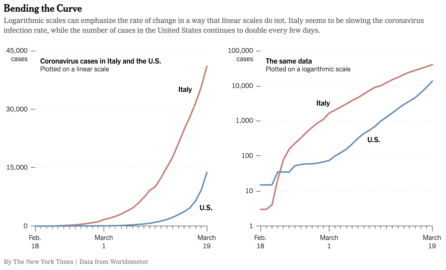
The two panels in Figure 23.1 show the same data about growing numbers of coronavirus cases, the left graph on linear axes, the right on the now-familiar semi-log axes.

Most people are excellent at comparing slopes, even if they find it difficult or tedious to quantify a slope with a number and units. For instance, a glance suffices to show that in the left graph, well through mid-March the red curve (Italy) is steeper on any given date than the blue curve (US). Correspondingly, the number of people with coronavirus was growing faster (per day) in Italy.

The right graph tells a different story: up until about March 1, the Italian cases were increasing faster than the US cases. Afterwards, the US sees a larger growth rate than Italy until, around March 19, the US growth rate is substantially larger than the Italy growth rate.

The previous two paragraphs and their corresponding graphs seem to contradict one another. But they are both accurate, truthful depictions of the same events. What’s different between the two graphs is that the left shows one kind of rate and the right shows another kind of rate. In the left, the slope is new-cases-per-day, the output of the derivative function

left graph: $\partial \mathrm{\_}t\text{daily\_new\_cases}(t)$.

On the right, the slope is the proportional increase in cases per day, that is,

right graph: $\frac{{\partial }_t\text{daily\_new\_cases}(t)}{\text{daily\_new\_cases}(t)}$.

From the chain rule, we know that

$${\partial }_t(\ln ((f(t)))=\frac{{\partial }_{t}f(t)}{f(t)}.$$

Since the right graph is on semi-log axes, the slope we perceive visually is ${\partial }_t(\ln (f(t)))$. That is an obscure-looking bunch of notation until the chain rule reveals it to be the rate of change in the number of covid cases at time $t$ divided by the number of cases at time $t$.

Tip 23.4: Deriving the chain rule using h-theory (optional)

The derivation of the chain rule relies on two closely related statements which are expressions of the idea that near any value $x$ a function can be expressed as a linear approximation with the slope equal to the derivative of the function :

1. $g(x+h)=g(x)+h{g}^{\prime }(x)$
2. $f(y+ϵ)=f(y)+ϵf^{\prime }(y)$, which is the same thing as (1) but uses $y$ as the argument name and $ϵ$ to stand for the small quantity we usually write with an $h$.

We will now look at ${\partial }_{x}f(g(x))$ by writing down the fundamental definition of the derivative. This, of course, involves the disclaimer $\underset{h\to 0}{lim}$ until we are sure that there is no division by $h$ involved.

$${\partial }_x\left(f(g(x))\right)\equiv \underset{h\to 0}{lim}\frac{f(g(x+h))-f(g(x))}{h}$$

Let’s examine closely the expression $f(g(x+h))$. Applying rule (1) above turns it into $$\underset{h\to 0}{lim}f(g(x)+h{g}^{\prime }(x))$$ Now apply rule (2) but substituting in $g(x)$ for $y$ and $h{g}^{\prime }(x)$ for $ϵ$, giving
$$\underset{h\to 0}{lim}f(g(x+h))=\underset{h\to 0}{lim}(f(g(x))+h{g}^{\prime }(x)f^{\prime }(g(x)))$$ We will substitute the $blue$ and $brown$ expression for the $magenta$ expression in $${\partial }_{x}f(g(x))\equiv \underset{h\to 0}{lim}\frac{f(g(x+h))-f(g(x))}{h}$$ giving $${\partial }_{x}f(g(x))\equiv \underset{h\to 0}{lim}\frac{f(g(x))+h{g}^{\prime }(x)f^{\prime }(g(x))-f(g(x))}{h}$$ In the denominator, $f(g(x))$ appears twice and cancels itself out. That leaves a single term with an $h$ in the numerator and an $h$ in the denominator. Those $h$’s cancel out, at the same time obviating the need for $\underset{h\to 0}{lim}$ and leaving us with the chain rule: $${\partial }_{x}f(g(x))\equiv \underset{h\to 0}{lim}\frac{h{g}^{\prime }(x)f^{\prime }(g(x))}{h}=f^{\prime }(g(x))g^{\prime }(x)$$