9 Assembling functions

When a modeler needs a new function for some purpose, there are three tactics. The best one depends on the circumstances and the availability of data.

Assemble the function from combinations of input-scaled pattern-book functions.

This tactic is well represented in Calculus textbooks. I think this is not so much a statement about the power of the tactic, but the general tendency to avoid working with data. For the applications of applied math, data is a valuable resource. When it’s available, as is often the case, there are alternatives to (1) that are available.

Use the data to guide the input and output scaling of pattern-book functions and their generalizations such as the power-law functions introduced in Section 5.2. This is often called “fitting the function”. We will study this tactic and its techniques in Chapter 11.
Split the domain of the desired function into small pieces. Then, for each piece, use very simple functions to capture the local behavior of a function locally. As the simple functions, the lower-order polynomaials x ~ a x or x ~a x + b or x ~ a x^ + b x^2 are widely used. The parameters are set entirely by data. This strategy was originally called “statistical learning,” then renamed “machine learning.” These days, “artificial intelligence” is used to refer to a particular strategy of iteration that slowly and gently incorporates data to tease the model parameters into a function that makes good predictions.

This chapter focusses on the mathematical framework for (1). Chapter 11 introduces the incorporation of data used in tactic (2). As for (3), we will need several core concepts of calculus as a basis for understanding, so we mainly defer the tactic to Chapter 49.

9.1 Linear combination

Section 8.4 introduced the notation of input and output scaling. For instance, Figure 11.6 illustrates how the pattern-book $\sin()$ function can be customized to model a particular situation. Recall that the input scaling involves inserting a straight-line function inside the parentheses, as in

\[f_1(t) \equiv \sin\left( a t + b\right) \tag{9.1}\]

You may recognize $at + b$ as a straight-line function. Possibly, your recognition would be easier if we wrote $at + b$ using different names for the input and the first parameter: $m x + b$. You have been trained to pronounce $m$ as the “slope” of the line and $b$ as the “y-intercept.”

Using both input and output scaling gives a more general kind of function:

\[f_2(t) \equiv A \sin(a t + b) + B \tag{9.2}\]

Math expression 9.2 is an example of a linear combination of two functions. The two functions are $g_1(t) \equiv 1$ and $g_2(t) \equiv sin(a t + b)$.

It might be easier to see Math expression 9.2 as a linear combination if the function were written explicitly using the two functions being combined, that is, as

\[f_2 \equiv A g_2(t) + B g_1(t)\]

The combination is made by scaling each of the functions involved then adding the scaled functions together. The two scaling factors, $A$ and $B$, could be called “parameters of $f_2()$,” which indeed they are. It would be good to get used to another word that’s used specifically for the parameters in a linear combination: “coefficients.” The advantage of “coefficients” as a name lies in it marking the parameters as those involved in a linear combination, rather than any of the other ways parameters can be used.

Note that “coefficients” always refers to parameters that are not inside the parentheses of a function. In contrast, often parameters are inside the parentheses as in Math expression 9.1. The parameters $a$ and $b$ in $\sin(a t + b)$ are inside the parentheses. Consequently, $a$ and $b$ shouldn’t be called “coefficients.” Sometimes, to emphasize this, parameters in parentheses are called “nonlinear parameters” to distinguish them from coefficients like $A$ and $B$.

To illustrate how linear combination is used to create new functions, consider polynomials, for instance, \[f(x) \equiv 3 x^2 + 5 x - 2\ . \tag{9.3}\] In high school, polynomials are often presented as puzzles—factor them to find the roots! In calculus, however, polynomials are used as functions for modeling. They are a kind of modeling “clay,” which can be shaped as needed.

There are three pattern-book functions in Math expression 9.3. In polynomials the functions being combined are all power-law functions: $g_0(x) \equiv 1$, $g_1(x) \equiv x$, and $g_2(x) \equiv x^2$. With these functions defined, we can write the polynomial $f(x)$ as \[f(x) \equiv 3 g_2(x) + 5 g_1(x) - 2 g_0(x)\] Each of the functions is being scaled by a quantity: 3, 5, and -2 respectively. Then the scaled functions are added up. That is a linear combination; scale and add.

Linear combination is an extremely important tactic that quantitative workers use throughout their careers. For instance, many physical systems are described by linear combinations. For instance, the motion of a vibrating molecule, a helicopter in flight, or a building shaken by an earthquake are described in terms of simple “modes” which are linearly combined to make up the entire motion. More down to Earth, the timbre of a musical instrument is set by the scalars in a linear combination of pure tones. And throughout work with data in science, commerce, government and other fields a primary data analysis method—called “regression”—is about finding the best linear combination of a set of explanatory variables to create a model function of the response variable.

Identical vs proportional vs straight-line

One of the pattern book functions is very simple; the output is identical to the input:

\[\text{identity}(x) \equiv x\] Multiplying the identity() function by a parameter gives a function that can well be called “proportional().”

\[\text{proportional}(x) \equiv a\ \text{identity}(x) = a\ x\] The parameter $a$ is often called the “constant of proportionality.”

It’s common to call this closely related function the “linear” function, but a better name is the “straight-line” function. “Straight-line” is the name we shall use in this book.

\[\text{straight\_line}(x) \equiv a\ x + b\]

9.2 Function composition

Function composition refers to combining functions by taking the input of one function and feeding it as input to another. “$g()$ composed with $h()$” means $g(h(x))$.

To illustrate, consider again the function defined in Math expression 9.2: \[f(t) \equiv A \sin\left( a t + b\right) + B\]

You’ve already seen how Math expression 9.2 is a linear combination of two functions $f_1(t) \equiv 1$ and $f_2(t) \equiv sin(a t + b)$. But $f_2()$ is not a linear combination. Instead, it is a function composition. The two functions being composed are $sin(x)$ and $a t + b$, producing $sin(a t + b)$. Here, $\sin()$ is the outer function in the composition and $at + b$ is the inner function.

In function composition, the order of the functions matters: $f(g(x))$ and $g(f(x))$ are in general completely different functions.

9.3 Function multiplication

Multiplication is the third in our repertoire of methods for making new functions. To review, here are the first two methods involving combining a function $f()$ with a function $g():

Linear combinations. Example: $n_1(t) \equiv 5 f(t) + 1.2 g(t)$.
Function composition. There are two possibilities which produce two distinct functions:
1. $c_1(t) \equiv f(g(t))$, that is, $g()$ is the inner function.
2. $c_2(t) \equiv g(f(t))$, that is, $g()$ is the outer function.

Now a new method:

Multiplication of the output of two functions. Example: $m(t)\equiv f(t) g(t)$. This is perfectly ordinary multiplication. Multiplication is commutative, as illustrated by the equality of $5 \times 2$ and $2 \times 5$. Owing to the commutativity of multiplication, it doesn’t matter whether $f()$ is first or $g()$ is first.

\[\underbrace{f(x) \times g(x)}_\text{multiplication}\ \ \ \ \underbrace{{\Large f(}g(x){\Large)} \ \ \text{or}\ \ \ {\Large g(}f(x){\Large)}}_\text{composition}\]

In function composition, only one of the functions—the interior function is applied to the overall input, $x$ in the above example. The exterior function is fed its input from the output of the interior function.

In multiplication, each of the functions is applied to the input individually. Then their outputs are multiplied to produce the overall output.

Application area 9.1 Modeling rise and fall

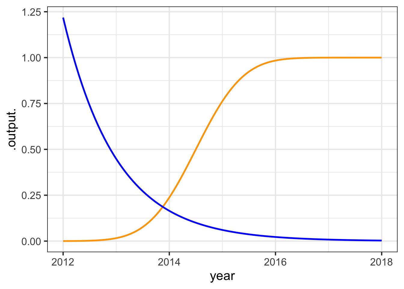
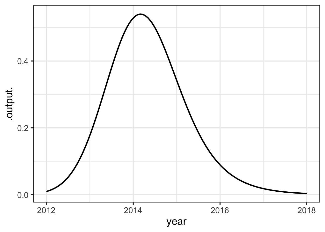
The initial rise in popularity of the social media platform Yik Yak was exponential. Then popularity leveled off, promising a steady, if static, business into the future. But, the internet being what it is, popularity collapsed to near zero and the company closed.

One way to model this pattern is by multiplying a sigmoid by an exponential. (See Figure 9.1.)

A sigmoid (orange) and an exponential function, shifted to be centered in mid-2014

Application area 9.2 Transient vibration

A guitar string is plucked to produce a note. The sound is, of course, vibrations of the air created by vibrations of the string.

After plucking, the note fades away. An simple model of this is a sinusoid (of the correct period to correspond to the frequency of the note) times a gaussian.

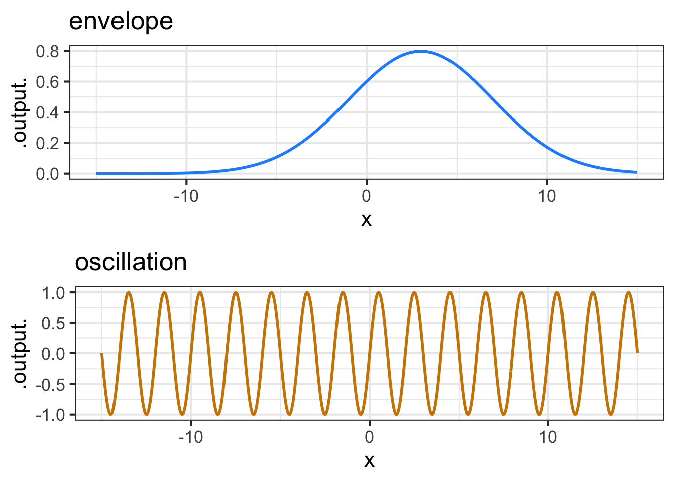
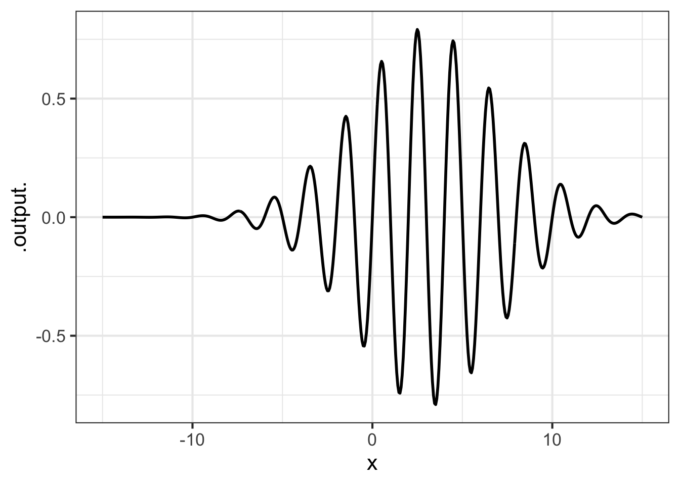
The two components of the wave packet: an envelope and an oscillation.

Function multiplication is used so often in modeling that you will see it in many modeling situations. Here’s one example that is important in physics and communication: the wave packet. Overall, the wave packet is a localized oscillation as in Figure 9.2. The packet can be modeled with the product of two pattern-book functions: a gaussian times a sinusoid.

9.4 Splitting the domain

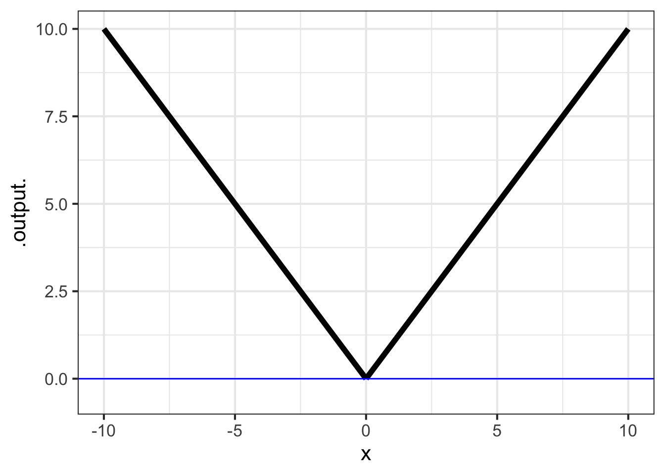
Consider the familiar absolute-value function, written \[\text{abs}(x) \equiv \left|x\right|\] in traditional notation. Written this way, the definition of abs() is a tautology: unless you already know what $\left|x\right|$ means, you will have no clue what’s going on.

Can we assemble abs() out of pattern-book functions? What’s distinctive about $abs(x)$ is the break at $x=0$. There is no similarly sharp transition in any of the pattern-book functions.

Defining a function piecewise, that is, constructing it from two different functions on two non-overlapping domains, provides the means to create a sharp transition. For the absolute value function, one domain is the negative inputs: $x < 0$. The other domain is the positive inputs: $0 \leq x$. Note that the domains do not overlap.

The absolute value function has two pieces, one to the left of input 0 for the function $-x$, the other to the right of 0 for the function $x$. The two pieces meet at input 0. \[\text{abs}(x) \equiv \left\{ \begin{array}{rl} x & \text{for}\ 0 \leq x \\ -x & \text{otherwise}\\\end{array} \right.\]

A function defined separately on different pieces of its domain is called a piecewise function. In the conventional mathematical notation, there is a large $\LARGE\left\{\right.$ followed by two or more lines. Each line gives a formula for that part of the function and indicates to which interval the formula applies.

Another piecewise function widely used in technical work, but not as familiar as $abs()$ is the Heaviside function, which has important uses in physics and engineering. \[\text{Heaviside}(x) \equiv \left\{ \begin{array}{cl} 1 & \text{for}\ 0 \leq x \\0 & \text{otherwise}\end{array} \right.\]

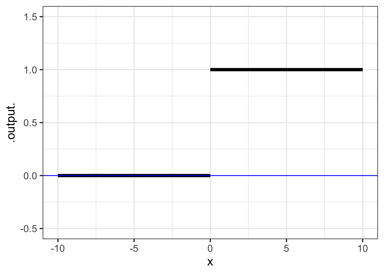
The Heaviside function is defined on the same two pieces of the number line as $abs()$. To the right of zero, Heaviside is identical to constant(). To the left, it is identical to 0 times constant$()$.

The vertical gap between the two pieces of the Heaviside function is called a discontinuity. Intuitively, you cannot draw a discontinuous function without lifting the pencil from the paper. The Heaviside’s discontinuity occurs at input $x=0$.

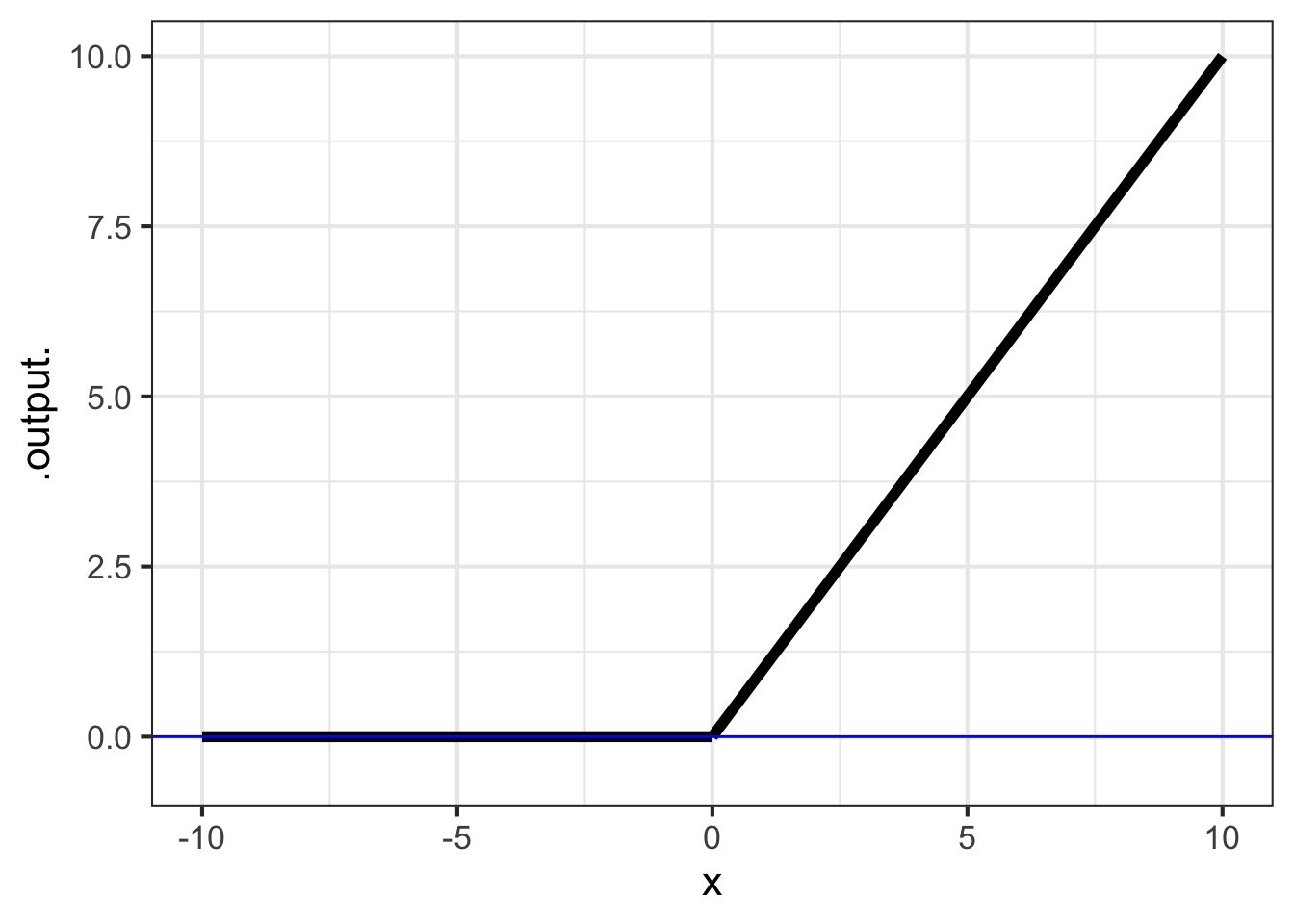
The ramp function is closely related to the Heaviside function. The ramp has output 0 when the input is negative. For positive inputs, the ramp is the identity function. \[\text{ramp}(x) \equiv \left\{ \begin{array}{rl} x & \text{for}\ 0 \leq x \\ 0 & \text{otherwise}\\\end{array} \right.\]

9.4.1 Computing notation

The usual mathematical notation for piecewise functions, spread out over multiple lines that are connected with a tall brace, is an obvious non-candidate for computer notation. In R, the stitching together of the two pieces can be done with the function ifelse(). The name is remarkably descriptive. The ifelse() function takes three arguments. The first is a question to be asked, the second is the value to return if the answer is “yes,” and the third is the value to return for a “no” answer.

To define abs() or Heaviside() the relevant question is, “Is the input on the right or left side of zero on the number line?” In widely-used computing languages such as R, the format for asking a question does not involve a question mark. For example, to ask the question, “Is 3 less than 2?” use the expression:

In mathematics notation, $3 < 2$ is a declarative statement and is an impossibility. More familiar would be $x < 2$, which is again a declarative statement putting a restriction on the possible values of the quantity $x$.

In computing notation, 3 < 2 or x < 2 is not a declaration, it is an imperative statement that directs the computer to do the calculation to find out if the statement is true or false for the particular values given.

Here’s a definition of Heaviside() written with ifelse().

Since Heaviside() is a function, the question $0 \leq x$ does not get answered at the time the function is defined. Instead, when the function is evaluated we will know the value of input $x$, can answer the $0 \leq x$ question, and use the answer to select either 1 or 0 as the output.

Table 9.1 shows computer notation for some common sorts of questions.

Table 9.1: Each of these imperative statements in R asks a question about numbers.

R notation	English
`x > 2`	“Is $x$ greater than 2?”
`y >= 3`	“Is $y$ greater than or equal to 3?”
`x == 4`	“Is $x$ exactly 4?”
`2 < x & x < 5`	“Is $x$ between 2 and 5?” Literally, “Is $x$ both greater than 2 and less than 5?”
`x < 2 \| x > 6`	“Is $x$ either less than 2 or greater than 6?”
`abs(x-5) < 2`	“Is $x$ within two units of 5?”

Application area 9.3 Heating with gas

Figure 9.6 is a graph of monthly natural gas use in the author’s household versus average temperature during the month. (Natural gas is measured in cubic feet, abbreviated ccf.)

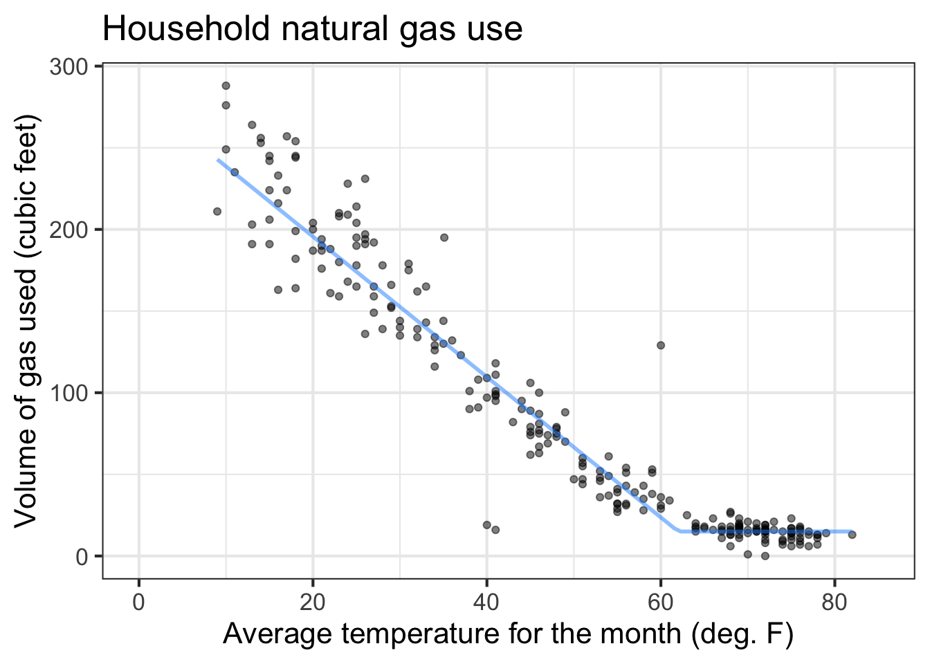
Figure 9.6: The amount of natural gas used for heating the author’s home varies with the outside temperature.

The graph looks somewhat like a hockey stick. A sloping straight-line dependence of ccf on temperature for temperatures below $60^\circ$F and constant for higher temperatures. The shape originates from the dual uses of natural gas. Gas is used for cooking and domestic hot water, the demand for which is more or less independent of outdoor temperature at about 15 ccf per month. Gas is also used for heating the house, but that is needed only when the temperature is less than about $60^\circ$F.

We can accomplish the hockey-stick shape with a linear combination of the ramp() function and a constant. The ramp function represents gas used for heating, the constant is the other uses of gas (which are modeled as not depending on temperature. Overall, the model is \[\text{gas}(x) \equiv 4.3\, \text{ramp}(62-x) + 15\ .\]

Note that the input to ramp() is 62 - $x$. This input scaling (Section 8.3) turns the ramp around so that it rises to the left. The transition between the flat and ramp sections occurs at $x=62$.

9.5 Computing outside the domain

Each of our pattern-book functions, with two exceptions, has a domain that is the entire number line $-\infty < x < \infty$. No matter how big or small is the value of the input, the function has an output. Such functions are particularly nice to work with since we never have to worry about the input going out of bounds.

The two exceptions are:

the logarithm function, which is defined only for $0 < x$.
some of the power-law functions: $x^p$.
- When $p$ is negative, the output of the function is undefined when $x=0$. You can see why with a simple example: $g(x) \equiv x^{-2}$. Most students had it drilled into them that “division by zero is illegal,” and $g(0) = \frac{1}{0} \frac{1}{0}$, a double law breaker.
- When $p$ is not an integer, that is $p \neq 1, 2, 3, \cdots$ the domain of the power-law function does not include negative inputs. To see why, consider the function $h(x) \equiv x^{1/3}$.

Division by zero on the computer

It can be tedious to make sure that you are on the right side of the law when dealing with functions whose domain is not the whole number line. The designers of the hardware that does computer arithmetic, after several decades of work, found a clever system to make it easier. It is a standard part of such hardware that whenever a function is handed an input that is not part of that function’s domain, one of two special “numbers” is returned. To illustrate:

sqrt(-3)
## [1] NaN
(-2)^0.9999
## [1] NaN
1/0
## [1] Inf

NaN stands for “not a number.” Just about any calculation involving NaN will generate NaN as a result, even those involving multiplication by zero or cancellation by subtraction or division.¹ For instance:

0 * NaN
## [1] NaN
NaN - NaN
## [1] NaN
NaN / NaN
## [1] NaN

Division by zero produces Inf, whose name is reminiscent of “infinity.” Inf infiltrates any calculation in which it takes part:

3 * Inf
## [1] Inf
sqrt(Inf)
## [1] Inf
0 * Inf
## [1] NaN
Inf + Inf
## [1] Inf
Inf - Inf
## [1] NaN
1/Inf
## [1] 0

To see the benefits of the NaN / Inf system let’s plot out the logarithm function over the graphics domain $-5 \leq x \leq 5$. Of course, part of that graphics domain, $-5 \leq x \leq 0$ is not in the domain of the logarithm function and the computer is entitled to give us a slap on the wrists. The NaN provides some room for politeness.

One that does produce a number is NaN^0.↩︎