13 Operations on functions
Chapters sec-parameters through sec-fitting-by-feature introduce concepts and techniques for constructing functions. This is an important aspect of building models, but it is not the only one. Typically, a modeler, after constructing appropriate functions, will manipulate them in ways that extract the information required to answer questions that motivated the modeling work. This chapter will introduce some of the operations and manipulations used to extract information from model functions.
There are five such operations that you will see many times throughout this book.
- Zero-finding: finding an input that produces the desired output. This is also called “inversion.”
- Optimization: finding an input that produces the largest output
- Iteration: building a result step-by-step
- Differentiation
- Integration (that is, Accumulation)
This chapter will introduce the first three of these. The remaining two—differentiation and integration—are the core operations of calculus. They will be introduced starting in Block II.
We take two different perspectives on the three operations: graphical and computational. Often, a graph lets you carry out an operation with sufficient precision for the purpose at hand. Graphs are relatively modern, coming into mainstream use only in the 1700s. Much of mathematics was developed before graphs were invented. It is often the case that the algebraic ways of implementing the operations are difficult, while graphical approaches can be very easy. This is especially true now that graphics are so easy to make. You can iterate (operation 3 above), zooming the graphics domain around an approximate answer.
Graphics connect well with human cognitive strengths, but the computer can also automatically carry out the operations quickly and precisely. The computing algorithms and software used for zero-finding/inversion and optimization are often based on concepts from calculus that we have not yet encountered. Software provides another advantage: Experts in a field can communicate with newbies so that anyone can use the operation in practice without necessarily developing a complete theoretical understanding of the algorithm. At this stage, before the calculus concepts have been introduced, our computational focus will be on how to set up the calculation and how to interpret the results.
Functions and operations
In computer languages, the word “function” is used to describe a piece of software which transforms inputs into an output. Examples of such software functions are making slice- and contour graphics, makeFun(), fitModel(), and so on. As well, we implement mathematical functions (using, for instance, makeFun()) as software functions.
Now that we are introducing operations on functions, we have a slight problem of nomenclature. The operations in this chapter are designed to be applied to mathematical functions represented as software functions. The software for these operations is also in the form of computer language functions. So, functions are being applied to functions. This can be confusing.
To avoid unnecessary confusion, we will write function, in monospaced font, when we are talking about a software implementation of operations such as those introduced in this chapter. As an example, the next section introduces an operation called “zero finding” to be applied to a function. The R/mosaic software that implements this operation is called Zeros(). That is, we apply the Zeros() function to a mathematical function such as \(h(z)\). In other words, for the purpose of extracting information from a function such as \(h(z)\), we will use a software function that carries out the information-extraction operation.
13.1 Zero finding
A function is a mechanism for turning any given input into an output. Zero finding is about going the other way: given an output value, find the corresponding input. As an example, consider the exponential function \(e^x\). Given a known input, say \(x=2.135\) you can easily compute the corresponding output as in Active R chunk lst-exp-213:
Depending on the modeling context, information can come in different forms. For instance, suppose the situation is:
- Given: We know that \(\exp(x_0) = 4.93\) for some as yet unknown \(x_0\).
- Information wanted: What is the value of \(x_0\)?
This sort of situation calls for “inverting” the \(\exp()\) function. There are very general and simple methods for performing this sort of extraction. We call these methods “zero finding. They involve searching for the value of an input that will make the output of a given function be zero.
Application area thm-earthquake Finding earthquakes and injured heart muscle.
We look at pretty simple functions in this book. But consider these two similar kinds of functions:
An earthquake occurs at some depth and location and involving a particular energy and direction of motion along the fault. The function is this: The motion creates waves that pass through the Earth’s crust and mantle and are refracted by the Earth’s core. In the end, they reach a seismometer at a geophysics research lab.
A heart attack has damaged some heart muscle. This alters the electrical activity of the heart. In every heart beat, the electrical activity passes as waves through the complex structure of the thorax and muscles, and on to the arms and legs. The function is this: how the alteration in activity appears when measured as electrical voltages on the surface of the body, as in an electro-cardiogram (ECG).
In both these cases, it’s possible to approximate the function. Often, this is done with simulation: building a detailed model of the Earth or a body and passing waves through the model. The inversion is the process of finding what input to the model produces the measured output.
Inverting algebraically
Some may already know a technique for finding the value of \(x_0\) in the Information/Extraction situation posed above. The process, learned in high-school algebra classes is to use the natural logarithm on the output 4.93.
How would you demonstrate that the result is correct? Feed the value you found for \(x_0\) back into the \(\exp()\) function and verify that you get 4.93.
This process works because we happen to have a function at hand, the natural logarithm, that is perfectly set up to “undo” the action of the exponential function. In high school, you learned a handful of function/inverse pairs: exp() and log() as you’ve just seen, sin() and arcsin(), square and square root, etc.
Memorizing the names of such function/inverse pairs is helpful in passing high-school algebra and for following derivations in texts and on the blackboard. But knowing the name is only part of the story. You have to be able to apply the functions to inputs. Typically, the only way you have to do this is with a machine such as a calculator or computer.
A similar high-school situations involves quadratic polynomials. Almost all readers will be familiar with this situation:
- Given: We know that \(x_0^2 - 3.9 x_0 = -7.2\) for some as yet unknown \(x_0\).
- Information wanted: What is the value of \(x_0\)?
High-school students learn to bring the \(-7.2\) to the left side of the equals sign and then find the “roots.” Applying the “quadratic formula” to the coefficients of the polynomial gives numerical values for the roots. which produces one or two numbers as a result. This is well and good so far as it goes, but the quadratic formula is no use for a slightly modified problem. For instance, suppose the situation is this:
- Given: We know that \(x_0^2 - 3.9 e^{x_0} = -7.2\) for some as yet unknown \(x_0\).
- Information wanted: What is the value of \(x_0\)?
Wouldn’t it be nice to have one simple technique that applies to all such problems? That’s what the zero-finding operation gives us.
Graphical zero-finding
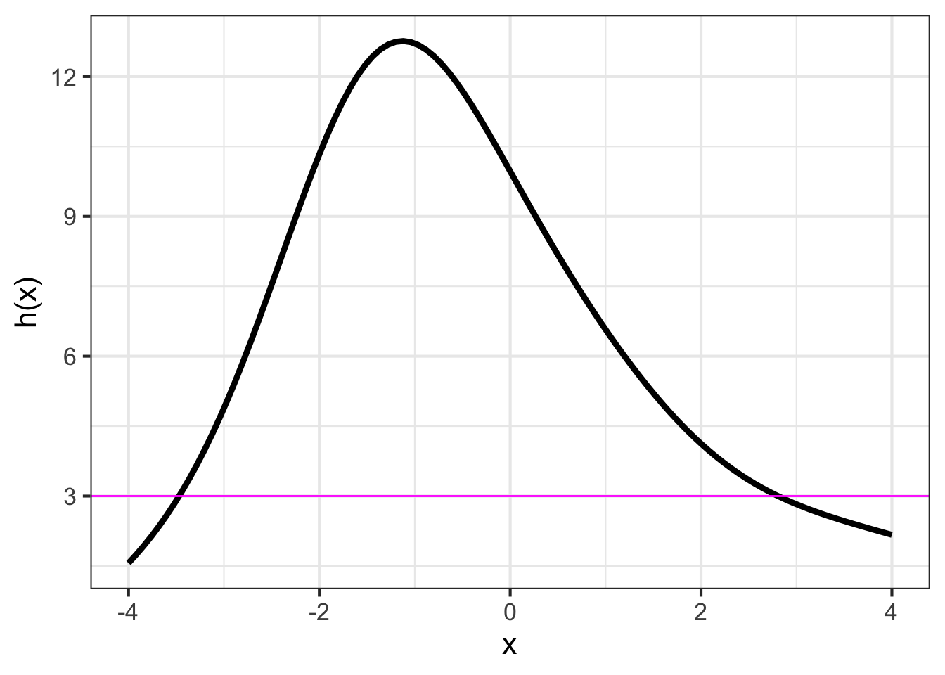
Consider any function \(h(x)\) that you constructed by linear combination and/or function multiplication and/or function composition. To illustrate, we will work with the function \(h(x)\) graphed in Figure fig-zero-finding1.
Suppose the output for which we want to find a corresponding input is 3, that is, we want to find \(x_0\) such that \(h(x_0)=3\).
The steps of the process are:
- Graph the function \(h(x)\) over a domain interval of interest.
- Draw a horizontal line located at the value on the right-hand side of the equation \(h(x_0) = 3\). (This is the magenta line in Figure fig-zero-finding1.)
- Find the places, if any, where the horizontal line intersects the graph of the function. In Figure fig-zero-finding1, there are two such values: \(x_0 = -3.5\) or \(x_0 = 2.75\).
Important 13.1: Graphical zero finding
A function \(g(t)\) is graphed below. Find a value \(t_0\) such that \(g(t_0) = 5\).
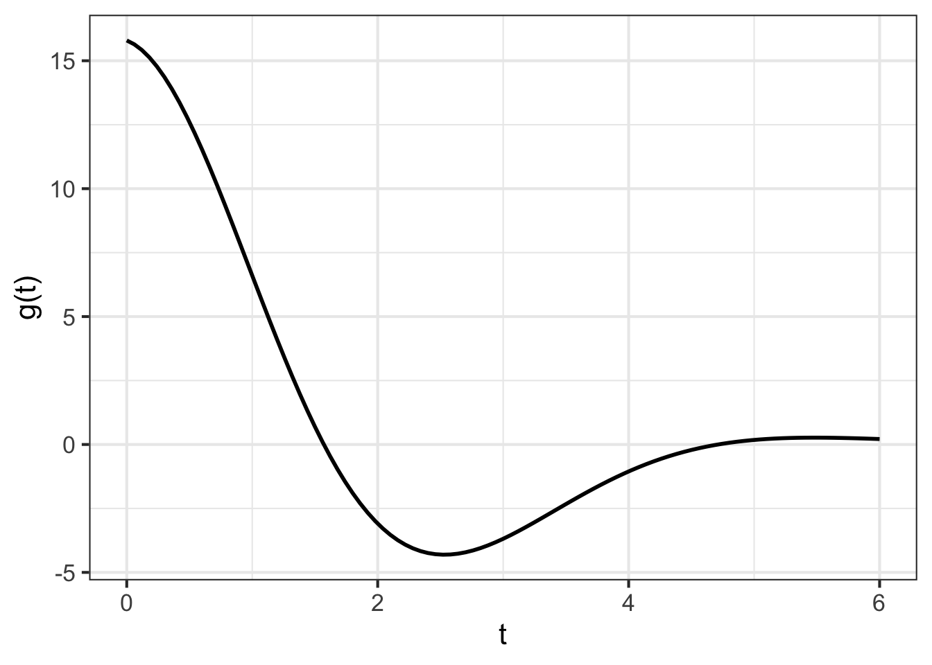
- Draw a horizontal line at output level 5.
- Find the t-value where the horizontal line intersects the function graph. There is only one such intersection and that is at about \(t=1.2\).
Consequently, \(t_0 = 1.2\), at least to the precision possible when reading a graph.
The graphical approach to zero finding is limited by your ability to locate positions on the vertical and horizontal axis. If you need more precision than the graph provides, you have two options:
Take a step-by-step, iterative approach. Use the graph to locate a rough value for the result. Then refine that answer by drawing another graph, zooming in on a small region around the result from the first step. You can iterate this process, repeatedly zooming in on the result you got from the previous step.
Use software implementing a numerical zero-finding algorithm. Such software is available in many different computer languages and a variety of algorithms is available, each with its own merits and demerits.
Numerical zero finding
In this book, for consistency with our notation, we use the R/mosaic Zeros() function. The first argument to Zeros() is a tilde expression and the second argument an interval of the domain over which to search.
Zeros() is set up to find inputs where the mathematical function defined in the tilde expression produces zero as an output. But suppose you are dealing with a problem like \(f(x) = 10\)? You can modify the tilde expression so that it implements a slightly different function: \(f(x) - 10\). If we can find \(x_0\) such that \(f(x_0) - 10 = 0\), that will also be the \(x_0\) satisfying \(f(x_0) = 10\).
Important 13.2: Computationally finding zeros
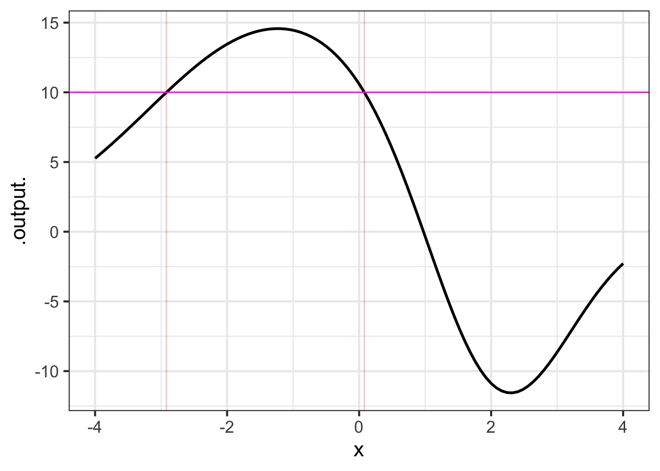
The point of this example is to show how to use Zeros(), so we will define a function \(f(x)\) using doodle_fun() from R/mosaic. This constructs a function by taking a linear combination of other functions selected at random. The argument seed=579 determines which functions will be in the linear combination. The function is graphed in Figure fig-doodle-579.
We want to find the zeros of the function \(f(x) - 10\) which corresponds to solving \(f(x) = 10\). The function Zeros() handles this for us.
The output produced by Zeros() is a data frame with one row for each of the \(x_0\) found. Here, two values were found: \(x_0 = -2.92\) and \(x_0 = 0.0795\), shown as vertical lines in Figure fig-doodle-579. The .output column reports \(f(x_0)\). In principal, this should be exactly zero. However, computer arithmetic is not always exactly precise. Even so, numbers as small as those in the .output. column—\(-3.4 \times 10^{-8}\) for example—are miniscule compared to the range of values seen in Figure fig-doodle-579.
13.2 Optimization
Optimization problems consist of both a modeling phase and a solution phase (that is, an information extraction phase). We use our knowledge of how the world works for the modeling phase. Then we extract information in the form we want from the solution phase.
In this chapter we will deal only with the solution phase. In real work, the modeling phase is essential
Graphical optimization
Simple. Look for local peaks, then read off the input that generates the value at the peak.
Numerical optimization
When it comes to functions, maximization is the process of finding an input to the function that produces a larger output than any of the other, nearby inputs.
To illustrate, Figure fig-show-peak1 shows a function f() with two peaks.
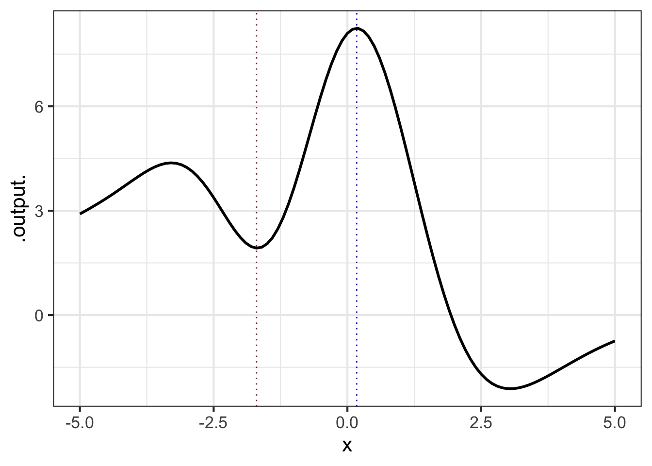
Just as you can see a mountain top from a distance, so you can see where the function takes on its peak values. Draw a vertical line through each of the peaks. The input value corresponding to each vertical line is called an argmax, short for “the argument1 at which the function reaches a local maximum value.
Minimization refers to the same technique, but where the vertical lines are drawn at the deepest point in each “valley” of the function graph. An input value located in one of those valleys is called an argmin.
Optimization is a general term that covers both maximization and minimization.
13.2.1 Numerical optimization
The R/mosaic argM() function finds a mathematical function’s argmax and argmin over a given domain. It works in exactly the same way as slice_plot(), but rather than drawing a graphic it returns a data frame giving the argmax in one row and the argmin in another. For instance, the function shown in Figure fig-show-peak1 is \(f()\), generated by doodle_fun():
The x column holds the argmax and argmin, the .output. column gives the value of the function output for the input x. The concavity column tells whether the function’s concavity at x is positive or negative. Near a peak, the concavity will be negative; near a valley, the concavity is positive. Consequently, you can see that the first row of the data frame corresponds to a local minimum and the second row is a local maximum.
argM() is set up to look for a single argmax and a single argmin in the domain interval given as the second argument. In Figure fig-show-peak1 there are two local peaks and two local valleys. argM() gives only the largest of the peaks and the deepest of the valleys.
13.3 Iteration
Many computations involve starting with a guess followed by a step-by-step process of refining the guess. A case in point is the process for calculating square roots. There isn’t an operational formula for a function that takes a number as an input and produces the square root of that number as the output. When we write \(\sqrt{\strut x}\) we aren’t saying how to calculate the output, just describing the sort of output we are looking for.
The function that is often used to calculate \(\sqrt{x}\) is better():
\[\text{better(guess)} = \frac{1}{2}\left( \text{guess} + \frac{x}{\text{guess}}\right)\ .\]
It may not be at all clear why this formula is related to finding a square root. Let’s put that matter off until the end of the section and concentrate our attention on how to use it.
To start, let’s define the function for the computer. Suppose we want to apply the square root function to the input 55, that is, calculate \(\sqrt{\strut x=55}\). The value we should assign to \(x\) is therefore 55.
Notice that \(x\) is cast in the role of a parameter of the function rather than an input to the function.
To calculate better(guess) we need an initial value for the guess. What should be this value and what will we do with the quantity better(guess) when we’ve calculated it.
Without explanation, we will use guess = 1. Calculating the output …
Neither our guess 1 nor the output 28 are \(\sqrt{\strut x=55}\). (Having long-ago memorized the squares of integers, we know \(\sqrt{\strut x=55}\) will be somewhere between 7 and 8. Neither 1 nor 28 are in that interval.)
The people—more than two thousand years ago—who invented the ideas behind the better() function were convinced that better() constructs a better guess for the answer we seek. It is not obvious why 28 should be a better guess than 1 for \(\sqrt{\strut x=55}\) but, out of respect, let’s accept their claim.
This is where iteration comes in. Even if 28 is a better guess than 1, 28 is still not a good guess. But we can use better() to find something better than 28:
To iterate an action means to perform that action over and over again. (“Iterate” stems from the Latin word iterum, meaning “again.”) A bird iterates its call, singing it over and over again. In mathematics, “iterate” has a twist. When we repeat the mathematical action, we will draw on the results of the previous angle rather than simply repeating the earlier calculation.
Continuing our iteration of better(), plugging the output of each calculation as the input for the next …
In the last step, the output of better() is practically identical to the input, so no reason to continue. We can confirm that the last output is a good guess for \(\sqrt{\strut x=55}\):
Graphical iteration
To iterate graphically, we graph the function to be iterated and mark the initial guess on the horizontal axis. For each iteration step, trace vertically from the current point to the function, then horizontally to the line of identity (blue dots). The result will be the starting point for the next guess.
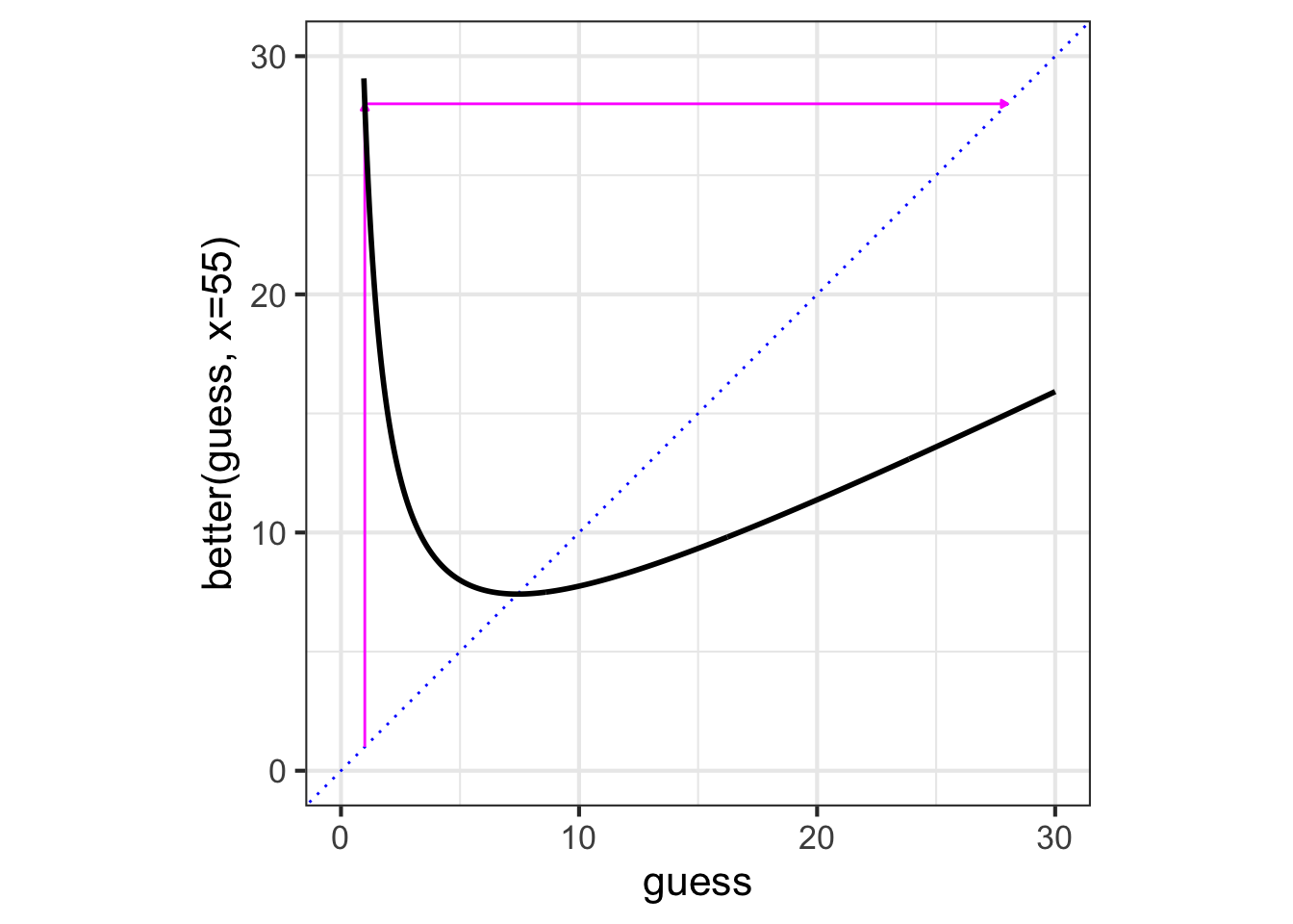
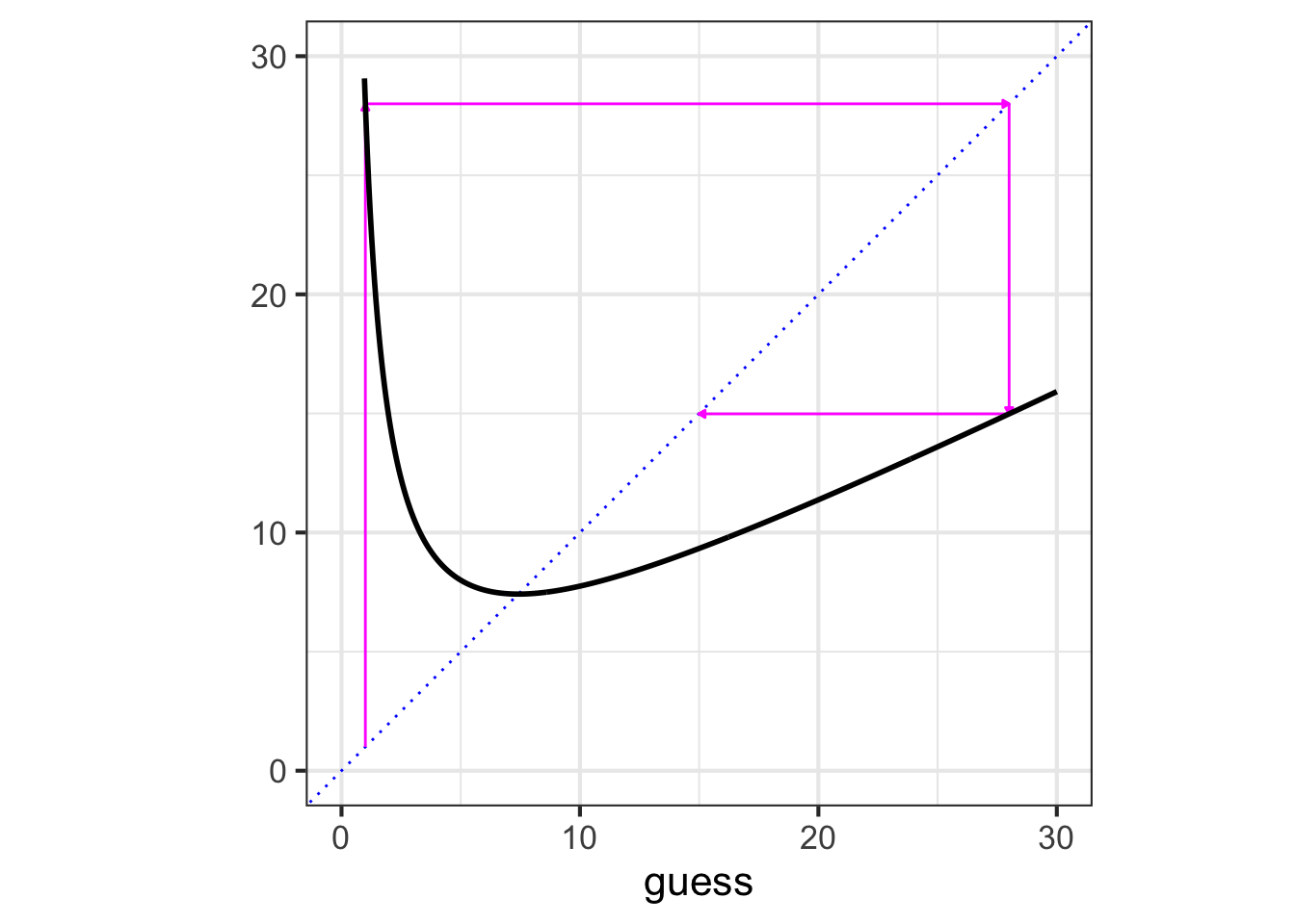
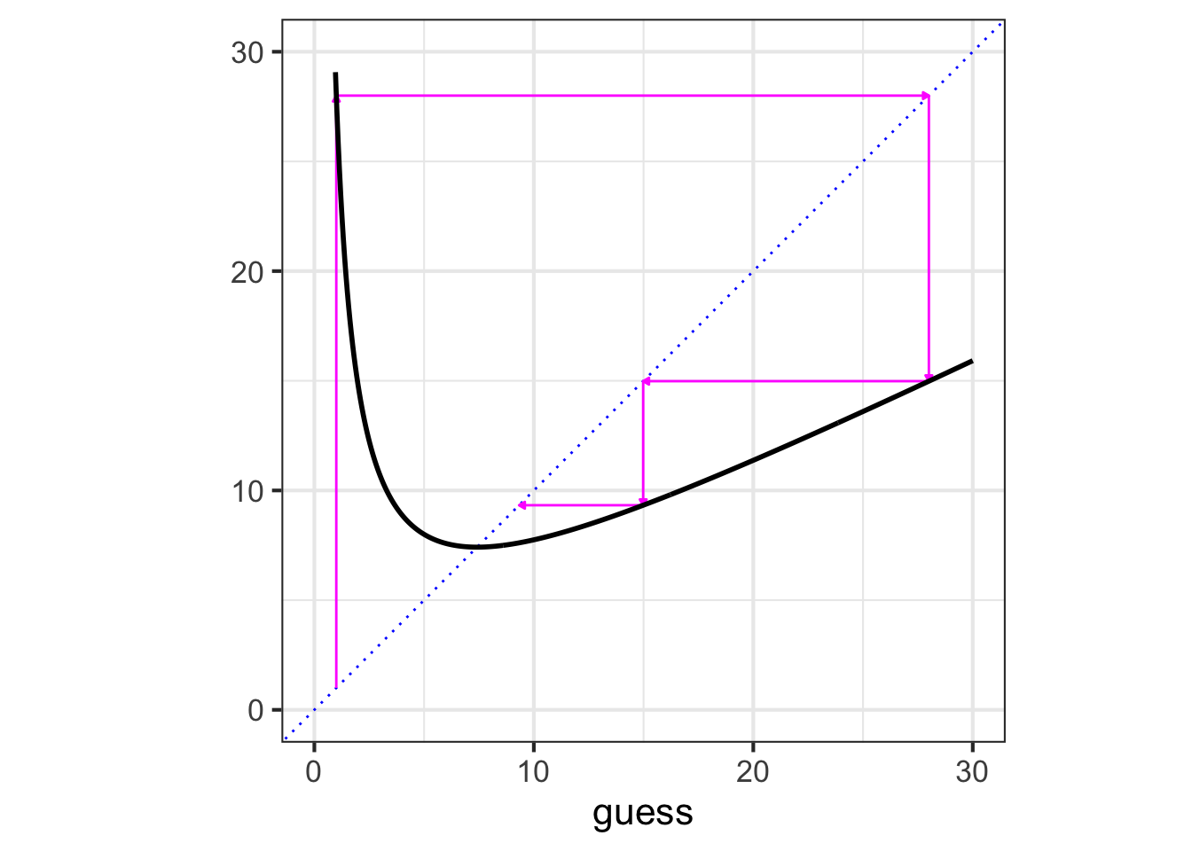
better() starting with an initial guess of 1.
Numerical iteration
Use the R/mosaic Iterate() function. The first argument is a tilde expression defining the function to be iterated. The second is the starting guess. The third is the number of iteration steps. For instance:
The output produced by Iterate() is a data frame. The initial guess is in the row with \(n=0\). Successive rows give the output, step by step, with each new iteration step.
Also known as an input.↩︎