21 Concavity and curvature
It is an easy visual task to discern the slope of a line segment. A glance shows whether the slope at that point is positive or negative. Comparing the slopes at two locales is also an automatic visual task: most people have little difficulty saying which slope is steeper. One consequence of this visual ability: it is easy to recognize whether a line that touches the graph at a point is tangent to the graph.
There are other aspects of functions, introduced in sec-concavity-intro, that are also readily discerned from a glance at the function graph.
- Concavity: We can tell within each locale whether the function is concave down, concave up, or not concave.
- Curvature: Generalizing the tangent line capability a bit, we can do a pretty good job of eyeballing the tangent circle or recognizing whether any given circle has too large or too small a radius.
- Smoothness: We can often distinguish smooth-looking functions from non-smooth ones. However, the trained eye can discern some kinds of mathematical smoothness but not others.
21.1 Quantifying concavity and curvature
It often happens in building models that the modeler (you!) knows something about the concavity or the curvature of a function. For example, concavity is essential in classical economics; the curve for supply as a function of price is concave down while the curve for demand as a function of price is concave up. For a train, car, or plane, sideways forces depend on the curvature of the track, road, or trajectory. Road designers need to calculate the curvature to know if the road is safe at the indicated speed.
It turns out that quantifying these properties of functions or shapes is naturally done by calculating second derivatives.
21.2 Concavity
Recall that to find the slope of a function \(f(x)\) at any input \(x\), you compute the derivative of that function, which we’ve been writing \(\partial_x\,f(x)\). Plug in some value for the input \(x\) and the output of \(\partial_x\, f(x)\) will be the slope of \(f(x)\) at that input. (sec-computing-derivs introduced some techniques for computing the derivative of any given function.)
Now we want to show how differentiation can quantify the concavity of a function. First, remember that when we speak of the “derivative” of a function, we mean the first derivative of the function. That full name naturally suggests that there will be a second derivative, a third derivative, and higher-order derivatives.
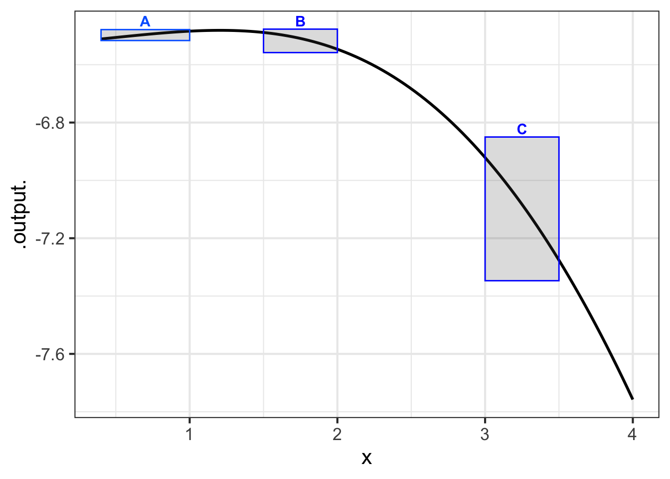
As introduced in sec-concavity-intro, the concavity of a function describes not the slope but the change in the slope. Figure fig-changing-slope2 depicts the slope of the function in each of the three boxes labelled A, B, and C. In the subdomain marked A, the function slope is positive, while in the subdomain B, the function slope is negative. This transition from the slope at A to the slope at B corresponds to the negative concavity of the function between A and B.
Similarly, the function’s concavity in the interval B to C reflects the transition in the instantaneous slope at B to the different instantaneous slope at C.
Let’s look at this using symbolic notation. Keep in mind that the function graphed is \(f(x)\) while the slope is the function \(\partial_x\,f(x)\). We’ve seen that the concavity is indicated by the change in slope of \(f()\), that is, the change in \(\partial_x\, f(x)\). We will go back to our standard way of describing the rate of change near an input \(x\):
\[\text{concavity.of.f}(x) \equiv\ \text{rate of change in}\ \partial_x\, f(x) = \] \[= \partial_x \left(\strut\partial_x f(x)\right) = \lim_{h\rightarrow 0}\frac{\partial_x f(x+h) - \partial_x f(x)}{h}\] We are defining the concavity of a function \(f()\) at any input \(x\) to be \(\partial_x \left(\strut\partial_x f(x)\right)\). We create the concavity_of_f(x) function by applying differentiation twice to the function \(f()\).
Such a double differentiation of a function \(f(x)\) is called the second derivative of \(f(x)\). The second derivative is so important in applications that it has its own compact notation: \[\text{second derivative of}\ f()\ \text{is written}\ \partial_{xx} f(x)\] Look carefully to see the difference between the first derivative \(\partial_x f(x)\) and the second derivative \(\partial_{xx} f(x)\): it is all in the double subscript \(_{xx}\).
Computing the second derivative is merely a matter of computing the first derivative \(\partial_x f(x)\) and then computing the (first) derivative of \(\partial_x f(x)\). In R this process looks like:
dx_f  <- D(   f(x) ~ x)   # First deriv. of f()
dxx_f <- D(dx_f(x) ~ x)   # Second deriv. of f()
A shortcut for second derivatives
A notation shortcut for the two-step process above: double up on the x on the right-hand side of the tilde:
dxx_f <- D(f(x) ~ x & x)
Read the ~ x & x as “differentiate by \(x\) and then once more by \(x\) again.”
21.3 Curvature
As you see from sec-concavity-deriv, it is easy to quantify the concavity of a function \(f(x)\): just evaluate the second derivative \(\partial_{xx} f(x)\). However, it turns out that people cannot do a good job of estimating the quantitative value of concavity by eye.
To illustrate, consider the square function, \(f(x) \equiv x^2\). (See Figure fig-square34.)
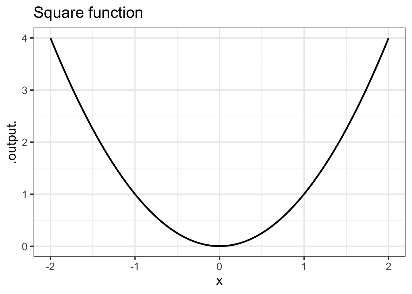
The square function is concave up. Now a test: Looking at the graph of the square function, where is the concavity the largest? Don’t read on until you’ve pointed where you think the concavity is largest.
Have you decided where the concavity is largest?
With your answer to the test question in mind, we can calculate the concavity of the square function using derivatives.
\[f(x) \equiv x^2\ \text{ so }\ \partial_x f(x) = 2 x\ \text{ and therefore }\ \partial_{xx} f(x) = 2\]
The second derivative of \(f(x)\) is positive, as expected for a function that is concave up. Surprisingly, however, the second derivative is constant.
The concavity-related property that the human eye reads from the function graph is not the concavity itself but the curvature of the function. The curvature of \(f(x)\) at \(x_0\) is defined to be the radius of the circle tangent to the function at \(x_0\).
Figure fig-inscribed-circles illustrates the changing curvature of \(f(x) \equiv x^2\) by inscribing tangent circles at several points on the function graph, marked with dots. That the function’s thin black line goes right down the middle of the broader lines used to draw the circles shows the tangency of the circle to the function graph.
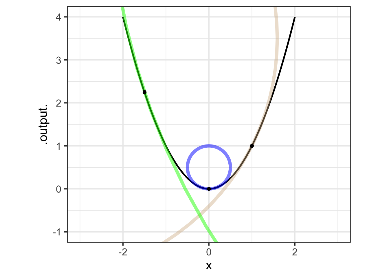
Black dots along the graph at the points indicate where the function graph is tangent to the inscribed circle. The visual sign of tangency is that the function graph goes right down the circle’s center.
The inscribed circle at \(x=0\) is tightest, the circle at \(x=1\) larger and the radius of the circle at \(x=-1.5\) is the largest of all. Whereas the concavity is the same at all points on the graph, the visual impression that the function is most highly curved near \(x=0\) is better captured by the radius of the inscribed circle. The radius of the inscribed circle at any point is the reciprocal of a quantity \({\cal K}\) called the curvature.
The curvature \({\cal K}\) of a function \(f(x)\) depends on both the first and second derivative. The formula for curvature \(K\) is somewhat off-putting; you are not expected to memorize it. But you can see where \(\partial x f()\) and \(\partial_{xx}f()\) come into play.
\[{\cal K}_f(x) \equiv \frac{\left|\partial_{xx} f(x)\right|}{\ \ \ \ \left|1 + \left[\strut\partial_x f(x)\right]^2\right|^{3/2}}\]
Mathematically, the curvature function \(\cal K()\) corresponds to the reciprocal of the radius of the tangent circle. When the tangent circle is tight, the output of \(\cal K()\) is large. When radius of the tangent circle is large, that is, when the function is very close to approximating a straight line, the output of \(\cal K()\) is very small.
Try it! try-curvature-of-square Calculate the curvature
Calculate the curvature of the square function: \(f(x) \equiv x^2\). Active R chunk lst-curvature-of-square will get you started by defining some of the functions needed:
Is the curvature constant as a function of \(x\)?
Hint
The formula for \(K()\) is
abs(dx_f(x))/abs(1 + (dxx_f(x)^2))^(2/3).