P <- makeFun(0.5*S + 0.5*T + 0.5*S*T - 0.5*S^2 ~ S & T)
contour_plot(P(S, T) ~ S & T, bounds(S=0:1, T=0:1))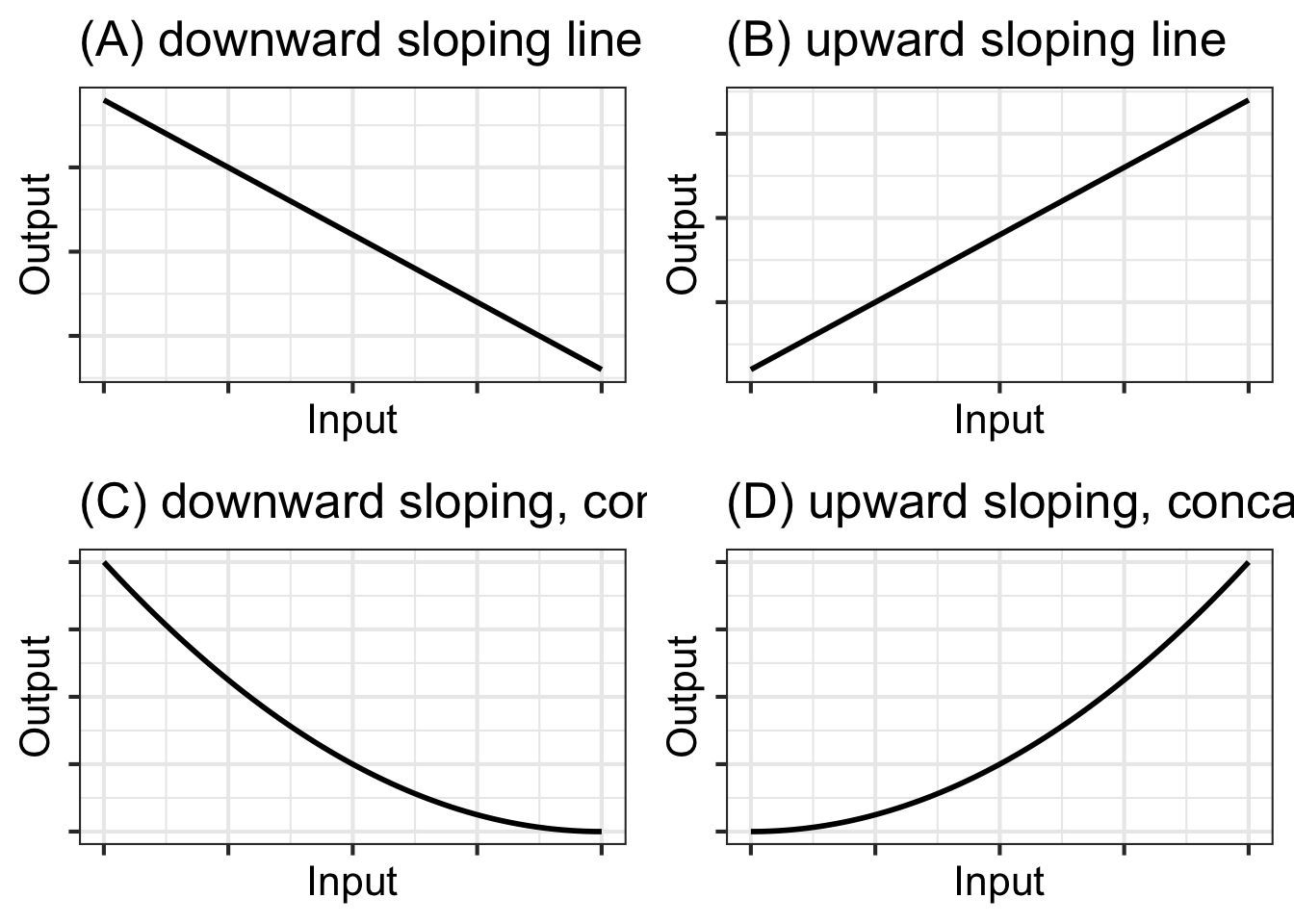
We have now encountered three concepts in Calculus that will prove a great help in building models.
Consider the problem of studying how plant growth is influenced by available water. It won’t be meaningful to compare tropical rain forests with high-latitude boreal forests. The availability of water is only one of many ways in which they differ. In a plant-growth experiment, one would hold the plant species and light exposure constant, and vary the water between specimens. In the language of partial differentiation, the result will be the partial derivative of growth rate with respect to water.
The expression for a general low-order polynomial in two inputs can be daunting to think about all at once: \[g(x, y) \equiv a_0 + a_x x + a_y y + a_{xy} x y + a_{xx} x^2 + a_{yy} y^2\] As with many complicated settings, a good approach can be to split things up into simpler pieces. With a low-order polynomial, one such splitting up involves partial derivatives. There are six potentially non-zero partial derivatives for a low-order polynomial, of which two are the same; so only five quantities to consider.
The above list states neutral mathematical facts that apply generally to any low-order polynomial whatsoever.1 Those facts, however, shape a way of asking questions of yourself that can help you shape the model of a given phenomenon based on what you already know about how things work.
To illustrate, consider the situation of modeling the effect of study \(S\) and of tutoring \(T\) (a.k.a. office hours, extended instruction) on performance \(P(S,T)\) on an exam. In the spirit of partial derivatives, we will assume that all other factors (student aptitude, workload, etc.) are held constant.
To start, pick fiducial values for \(S\) and \(T\) to define the local domain for the model. Since \(S=0\) and \(T=0\) are easy to envision, we will use those for the fiducial values.
Next, ask five questions, in this order, about the system being modeled.
Now the questions get a little bit harder and will exercise your calculus-intuition since you will have to think about changes in the rates of change.
The other way round, \(\partial_S \left[\partial_T P(S,T) \right]\) is a matter of whether increasing study will enhance the positive effect of tutoring. We will say yes here again, because a better knowledge of the material from studying will help you follow what the tutor is saying and doing. From pure mathematics, we already know that the two forms of mixed partials are equivalent, but to the human mind they sometimes (and incorrectly) appear to be different in some subtle, ineffable way.
In some modeling contexts, there might be no clear answer to the question of \(\partial_{xy}\, g(x,y)\). That is also a useful result, since it tells us that the \(a_{xy}\) term may not be important to understanding that system.
On to the question of \(\partial_{SS} P(S,T)\), that is, whether \(a_{SS}\) is positive, negative, or negligible. We know that \(a_{SS} S^2\) will be small whenever \(S\) is small, so this is our opportunity to think about bigger \(S\). So does the impact of a unit of additional study increase or decrease the more you study? One point of view is that there is some moment when “it all comes together” and you understand the topic well. But after that epiphany, more study might not accomplish as much as before the epiphany. Another bit of experience is that “cramming” is not an effective study strategy. And then there is your social life … So let’s say, provisionally, that there is an argmax to study, beyond which point you’re not helping yourself. This means that \(a_{SS} < 0\).
Finally, consider \(\partial_{TT} P(S, T)\). Reasonable people might disagree here, which is itself a reason to suspect that \(a_{TT}\) is negligible.
Answering these questions does not provide a numerical value for the coefficients on the low-order polynomial, and says nothing at all about \(a_0\), since all the questions are about change.
Another step forward in extracting what you know about the system you are modeling is to construct the polynomial informed by questions 1 through 5. Since you don’t know the numerical values for the coefficients, this might seem impossible. But there is a another modeler’s trick that might help.
To get started, consider the domains of both \(S\) and \(T\) to be the interval zero to one. This is not to say that we think one hour of study is the most possible but simply to defer the question of what are appropriate units for \(S\) and \(T\). Very much in this spirit, for the coefficients we will use \(+0.5\) when are previous answers indicated that the coefficient should be greater than zero, \(-0.5\) when the answers pointed to a negative coefficient, and zero if we don’t know. Using this technique, here is the model, which mainly serves as a basis for checking whether our previous answers are in line with our broader intuition before we move on quantitatively.
P <- makeFun(0.5*S + 0.5*T + 0.5*S*T - 0.5*S^2 ~ S & T)
contour_plot(P(S, T) ~ S & T, bounds(S=0:1, T=0:1))
Notice that for small values of \(T\), the horizontal spacing between adjacent contours is large. That is, it takes a lot of study to improve performance a little. At large values of \(T\) the horizontal spacing between contours is smaller.
Low-order polynomials are often used for constructing functions from data. In this section, I’ll demonstrate briefly how this can be done. The full theory will be introduced in Block 5 of this text.
The data I’ll use for the demonstration is a set of physical measurements of height, weight, abdominal circumference, etc. on 252 human subjects. These are contained in the Body_fat data frame, shown below.
One of the variables records the body-fat percentage, that is, the fraction of the body’s mass that is fat. This is thought to be an indicator of fitness and health, but it is extremely hard to measure and involves weighing the person when they are fully submerged in water. This difficulty motivates the development of a method to approximation body-fat percentage from other, easier to make measurements such as height, weight, and so on.
For the purpose of this demonstration, we will build a local polynomial model of body-fat percentage as a function of height (in inches) and weight (in pounds).
The polynomial we choose will omit the quadratic terms. It will contain the constant, linear, and interaction terms only. That is \[\text{body.fat}(h, w) \equiv c_0 + c_h h + c_w w + c_{hw} h w\] The process of finding the best coefficients in the polynomial is called linear regression. Without going into the details, we will use linear regression to build the body-fat model and then display the model function as a contour plot.
mod <- lm(bodyfat ~ height + weight + height*weight,
          data = Body_fat)
body_fat_fun <- makeFun(mod)
contour_plot(body_fat_fun(height, weight) ~ height + weight,
             bounds(weight=c(100, 250), height = c(60, 80))) %>%
  gf_labs(title = "Body fat percentage")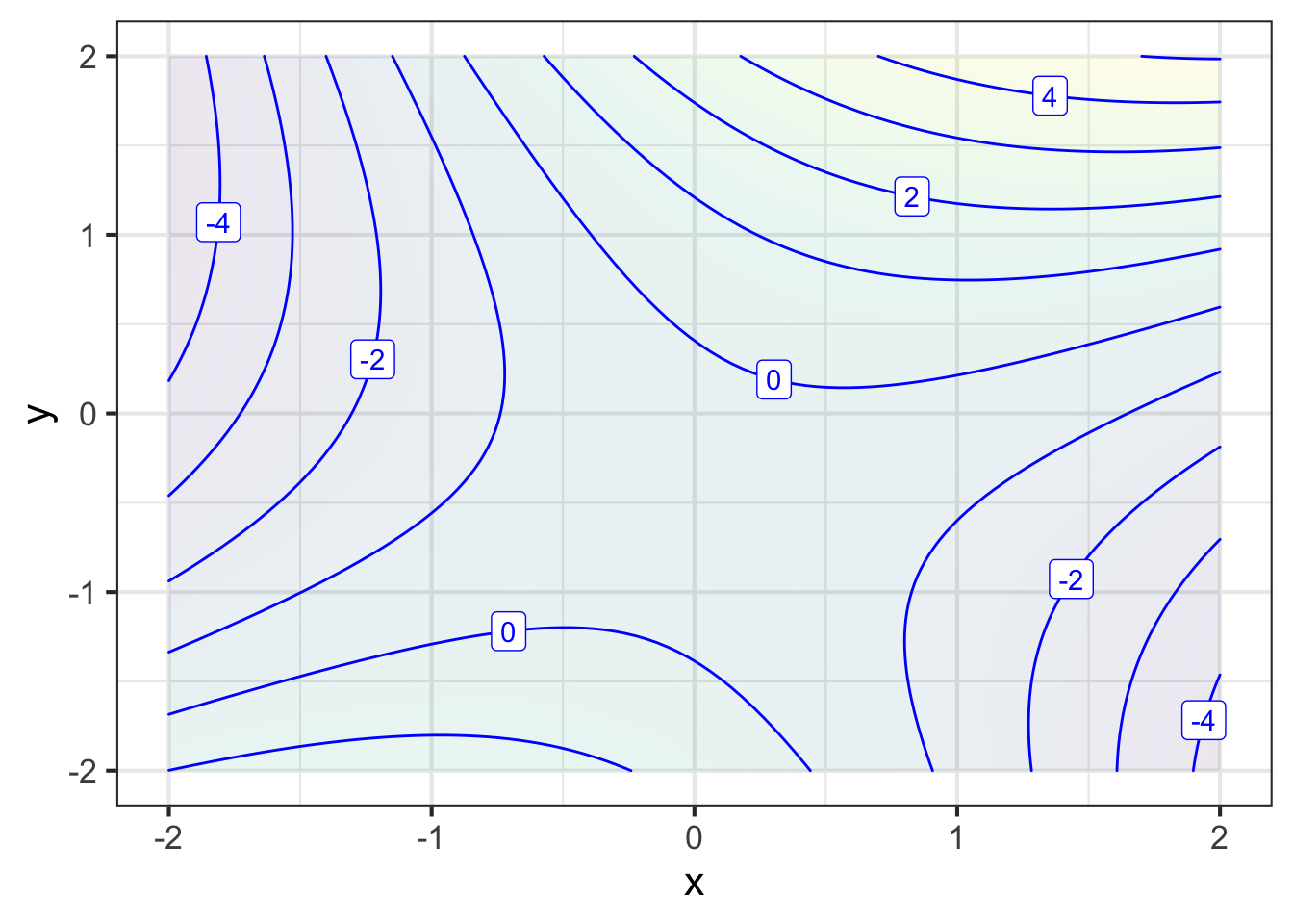
Block 3 looks at linear regression in more detail.
Note that any other derivative you construct, for instance \(\partial_{xxy} g(x,y)\) must always be zero.↩︎