1 Quantity, function, space
One good definition1 of “mathematics” is “the abstract science of number, quantity, and space.” The chapter title, however, doesn’t include the word “number.” Why not? The answer lies in another word in the definition: “abstract.”
“Abstract” means “based on general ideas and not on any particular person, thing, or situation.” Numbers are abstract; they can be used to represent all sorts of things, sheep, blood pressure, age, and so on without end. The mechanics of working with numbers is the same regardless of the kind of thing involved. In other words, abstract.
This book is about applied mathematics: the topics and methods of mathematics that are particularly useful in representing—that is, “modeling”—particular objects or situations. The topics and methods of applied mathematics are abstract in the sense that they can be usefully applied to a huge range of situations. For this book, we have carefully selected topics that are particulary useful in modeling situations and drawing conclusions from those models.
As mentioned previously, a “model” is a representation of an object or situation for a given purpose. A blueprint is a model of a building. A doll is a model of a person. We construct models because they are easier to manipulate than the real object being represented. Want to take down a wall between rooms? To do this in the blueprint model doesn’t require sweat or a sledgehammer; just erase the lines corresponding to the wall. Time to play? Just take the doll out of the toy chest and you’re ready to go.
We will focus on mathematical models, the kind of model made out of mathematical concepts and constructs. Three of these are listed in the chapter title, but there are others we will encounter later. Mathematical models make it particularly easy to perform manipulations such as asking and answering “what if” questions, predicting outcomes, and creating effective designs of objects and mechanisms. A good example is the use of spreadsheet software to figure out a budget.
As you know, a spreadsheet is a device for calculating with numbers. The word “calculate” comes from the Latin “calculus” which originally meant “stone” or “pebble.” Thousands of years before spreadsheets were invented, people were using tables with divots holding pebbles. Moving the pebbles around was the mechanism for calculation. An “abacus” is a particularly clever re-arrangement that replaces the pebbles with beads on a stick. For the last 250 years, however, “Calculus” has come to refer to a set of mathematical concepts and techniques that emerged as part of the Enlightenment and proved spectacularly useful for creating and manipulating mathematical models in physics, chemistry, engineering, and a host of other fields such as economics.
1.1 Quantity vs number
A mathematical quantity is an amount. How we measure amounts depends on the kind of stuff we are measuring. The real-world stuff might be time, speed, force, price inflation, physiological and ecological systems … anything to which arithmetic can be applied!
Everyone learns that arithmetic provides a set of patterns and rules for manipulating numbers. A number is a special, abstract kind of quantity. Among people who work with applied mathematics, experience has shown that numbers lack something that is important in many modeling situations: units. To fill the gap, we use “quantity” to indicate a structure with two parts: (1) a number and (2) the units of measurement. From this perspective, a number is merely a quantity that has no units.
We learn about units in elementary school, where we study the kinds of units appropriate for measuring tangible stuff. For example, the capacity of a water bottle might be presented in liters, cups, fluid ounces, gallons, bushels, and so on. The area of a field or apartment can be measured in square-meters, hectares, square-feet, square yards, acres, and so on. One of the things school-children learn about units is to identify what kind of stuff is measured by any given unit. For example, a gallon and a cup measure the same kind of stuff: volume. A meter and an inch measure the same kind of stuff: length. Some students also learn how to convert between units. For example, a meter is about 40 inches, a gallon is exactly 16 cups and a cup is exactly 48 teaspoons. But there is no way to convert, say, an inch into a cup. These lessons on units are useful in everyday life, even if most adults have only a limited recollection of them.
Moving beyond stuff like length, area, volume, and time can be difficult. You probably recognize kilometers-per-hour (or miles-per-hour) as a unit of velocity, but many student struggle when they first encounter something like meters-per-second-per-second, which is a unit for acceleration.
One of the great uses of Calculus is to convert between different kinds of stuff. A simple, everyday example is relevant to transportation. You can convert from speed (say, miles-per-hour) to distance travelled. The conversion is accomplished by multiplying speed by the duration of movement. Or, for some purposes, you might need to convert into speed two different measurements: distance travelled and time taken. In later chapters, we will encounter many situations where such conversions between types of stuff is important.
Keeping track of the type of stuff is an important habit when using Calculus for such conversions. In other words, you need to keep track of the units of each kind of stuff.
When talking about the methods of Calculus, however, there is a shorthand that enables you to see what kind of conversion is being done. This shorthand can help you select the appropriate arithmetical or Calculus method for whatever model manipulation you need to do, and it is especially helpful for spotting and correcting errors. The shorthand involves explicitly noting the “dimension” of the quantity.
Units and dimensions are closely related. Knowing the units, you can readily figure out the dimension. But knowing the dimension makes it easier to design and check your calculations. sec-dimensions-and-units will describe units and dimension more thoroughly. For now, however, we will give just a hint, enough to understand why knowing and understanding dimensions will help tremendously in your calculation.
In particular, we want to emphasize the reason to think about using quantities rather than mere numbers. Whenever you see a quantity, you should expect to see units or their shorthand, dimension.
Although there are hundreds of different kinds of units, we will need only four basic dimensions for most of the applications presented in this book. These are:
- time, denoted T
- length, denoted L
- mass, denoted M
- money, denoted V (for “value”)
Consider the familiar rules of arithmetic. The basic actions—addition, subtraction, multiplication, division—apply to any two numbers (although division by zero is not allowed). So 17 + 1.3 is 18.3, whatever those numbers are meant to represent. But the two quantities 17 inches and 1.3 seconds (L and T, respectively) cannot be meaningfully added. To apply addition and subtraction, the two quantities must be in the same unit, hence the same dimension. If you encounter someone adding quantities with different dimensions, you know you have spotted an error.
On the other hand, division and multiplication can work with any two quantities, regardless of their respective dimensions. In fact, division and multiplication are the basic arithmetic that enables us to construct new kinds of stuff from old kinds of stuff. For insight into the use of the word “dimension,” consider that a length times a length (L \(\times\) L) gives an area (L2) and an area times a length (L2 \(\times\) L) gives a volume (L^3). These correspond to one-, two- and three-dimensional objects respectively.
The mathematics of units and dimension are to the technical world what common sense is in our everyday world. For instance (and this may not make sense at this point), if people tell me they are taking the square root of 10 liters, I know immediately that either they are just mistaken or that they haven’t told me essential elements of the situation. It is just as if someone said, “I swam across the tennis court.” You know that person either used the wrong verb—walk or run would work—or that it wasn’t a tennis court, or that something important was unstated, perhaps, “During the flood, I swam across the tennis court.”
1.2 Functions
Functions, in their mathematical and computing sense, are central to calculus. The introduction to this Preliminaries Block states, “Calculus is about change, and change is about relationships.” The idea of a mathematical function gives a definite perspective on this. The relationship represented by a function is between the function’s input and the function’s output. The input might be day-of-year2 and the output cumulative rainfall up to that day. Every day it rains, the cumulative rainfall increases.
The input is the altitude on your hike up Pikes Peak to its peak elevation of 14,115 feet; the output is the air temperature. Typically, as you gain altitude the temperature goes down.
The input is the number of hours past noon; the output is the brightness of sunlight. As the afternoon progresses, the light grows dimmer, but only to a point.
A function is a mathematical concept for taking one or more inputs and returning an output. In calculus, we will deal mainly with functions that take one or more quantities as inputs and return another quantity as output.
Be aware of our use of “input” and “output” in place of the vague, but commonly used, “variable.” Try to put the word “variable” out of mind for the present, until we get to discussing the nature of data.
But sometimes we will work with functions that take functions as input and return a quantity as output. And, perhaps surprisingly, there will be functions that take a function as an input and return a function as output.
In a definition like \(f(x) \equiv \sqrt{\strut x}\), think of \(x\) as the name of an input. So far as the definition is concerned, \(x\) is just a name. We could have used any other name; it is only convention that leads us to choose \(x\). The definition could equally well have been \(f(y) \equiv \sqrt{\strut y}\) or \(f(\text{zebra}) \equiv \sqrt{\strut\text{zebra}}\).
Notation like \(f(x)\) is also used for something completely different from a definition. In particular, \(f(x)\) can mean apply the function \(f()\) to a quantity named \(x\). You can always tell which is intended—function definition or applying a function—by whether the \(\equiv\) sign is involved in the expression.
Later in this Preliminaries Block, we will introduce the “pattern-book functions.” These always take a pure number as input and return a pure number as output. In the Modeling Block, we will turn to functions that take quantities—which generally have units—as input and return another quantity as output. The output quantity also generally has units.
One familiar sign of applying a function is when the contents of the parentheses are not a symbolic name but a numeral. For example, when we write \(\sin(7.3)\) we give the numerical value \(7.3\) to the sine function. The sine function then does its calculation and returns the value 0.8504366. In other words, \(\sin(7.3)\) is utterly equivalent to 0.8504366.
In contrast, using a name on it is own inside the parentheses indicates that the specific value for the input is being determined elsewhere. For example, when defining a function we often will be combining two or more functions, like this: \[g(x) \equiv \exp(x) \sin(x)\] or \[h(y,z) \equiv \ln(z) \left(\strut\sin(z) - \cos(y)\right)\ .\] The \(y\) and \(z\) on the left side of the definition are the names of the inputs to \(h()\).3 The right side describes how to construct the output, which is being done by applying \(\ln()\), \(\sin()\) and \(\cos()\) to the inputs. Using the names on the right side tells us which function is being applied to which input. We won’t know what the specific values those inputs will have until the function \(h()\) is being applied to inputs, as with \[h(y=1.7, z=3.2)\ .\]
Once we have specific inputs, we (or the computer) can plug them into the right side of the definition to determine the function output: \[\ln(3.2)\left(\sin(3.2) - \strut \cos(1.7)\right) = 1.163(-0.0584 + 0.1288) =-0.2178\ .\]
sec-space-intro introduces the idea of “spaces.” A function maps each point in the function’s input space into a single point in the function’s output space. The input and output spaces are also known respectively as the “domain” and “range” of the function.
1.3 Spaces
Calculus is largely about change, and change involves movement. To move, as you know, means to change location. But we often use location as a metaphor for other things. Consider, for example, the everyday expression, “The temperature is getting higher.” This is not pointing to a thermometer rising up in the air, but to a quantity as it changes.
To represent a quantity as it changes we need to provide scope for movement. One way to do this is familiar from schooling: the number line. Each location on the number line corresponds to a possible value for a quantity. The particular value of that quantity at a specific moment in time is represented as a tiny bead on that line. The line as a whole encompasses many other locations. The changing quantity is the movement of the bead.
Figure fig-number-line-1 shows a number line as conventionally drawn. I have placed two different colored dots on the line to correspond to two different quantities: \(\color{blue}{6.3^\circ\ \text{C}}\) and \(\color{magenta}{-4.5^\circ \text{C}}\). (You only know that the line is about temperature because I told you.)

The graphical element representing the set of possibilities is the horizontal line segment. The tick marks and labels are added to enable you to translate any given location into the corresponding quantity. In mathematics texts, it’s common to put arrowheads at the ends of the line segment, perhaps to remind you that a line is infinite in length. But in other disciplines, no infinity or arrowheads are needed: the picture is just a scale to help people translate location into quantity.
I could have placed many dots on the line to represent many different particular quantitities. Of course, all the dots would be representing temperatures in \(^\circ\text{C}\) since that is the sort of quantity that the number line in Figure fig-number-line-1 represents.
A more general way for representing pairs of quantities is the coordinate plane, which Figure fig-coordinate-plane shows in the mathematics-text style. (sec-graphs-and-graphics switches to another style more commonly used across disciplines.)
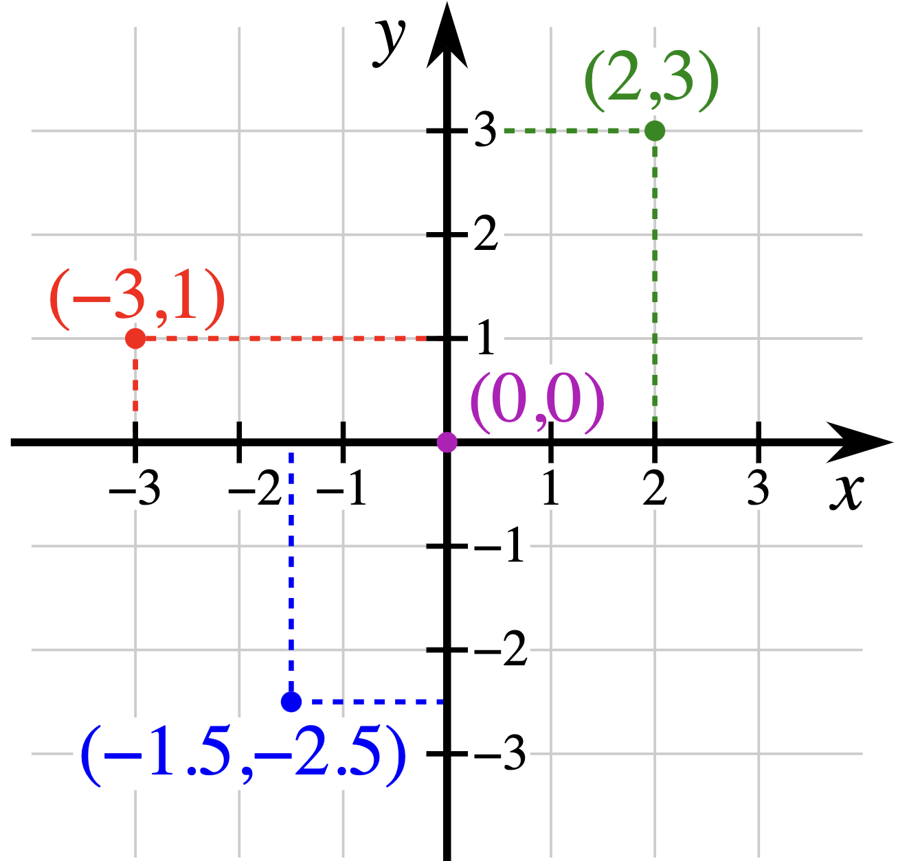
Every location in the coordinate plane is a possibility. A specific pair of quantities is displayed by placing a dot. Figure fig-coordinate-plane has four such dots, corresponding to four distinct pairs of quantities.
The space annoted by the coordinate axes and grid is two-dimensional, analogous to a table-top or a piece of paper or a computer display’s surface. Two-dimensional space accommodates change in each of the two quantities.
Everyday life acquaints us well with three-dimensional spaces, where each location corresponds to a possible value for each of three quantities. Displaying a three-dimensional space is difficult to do well because conventional displays show only two dimensions. Figure fig-three-coordinates shows one style that uses perspective and shading to create the impression of a 3-D scene.
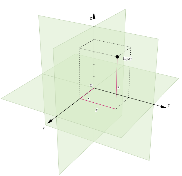
Drawings of one-dimensional space (Figure fig-number-line-1) or two-dimensional space (Figure fig-coordinate-plane) make it straightforward to read off the quantitative value corresponding to any location. Already in 3-dimensional space, reading quantitative coordinates is difficult and requires conscious mental effort. We will make only limited use of 3-D displays.
Consider now what the different dimensional spaces permit in terms of movement, that is, how quantities can change. The number line permits one kind of movement, left-right in Figure fig-number-line-1. Even though we use two words to name the kind of movement—“left” and “right”—we still consider movement in either opposing direction as one kind of movement. Left is the opposite of right. The coordinate plane permits two kinds of movement: left-right and up-down. A three-dimensional space permits three kinds of movement: left-right, up-down, nearer-farther. We often say that each type of movement is along an axis. as is conventional for one- and two-dimensional spaces. The number line has one axis, the coordinate plane has two axes, and three-dimensional space has three.
Figures fig-number-line-1, fig-coordinate-plane, and fig-three-coordinates are conventional drawings of one-, two-, and three-dimensional spaces respectively. What about four- or higher-dimensional spaces? Many people put their foot down here and refuse to accept such a thing. Some others will point to the Theory of Relativity where an essential concept is “space-time,” a four-dimensional space sometimes denoted as \((x, y, z, t)\). True though this be, it does not much appeal to intuition and for a good reason. We are free to move objects in their x-, y-, and z-coordinates, but we have no control over time.
Engineers, statisticians, physicists, and others often use the phrase “degree of freedom” to refer to a type of movement. In English, we have many phrases for different types of movement: in-and-out, back-and-forth, clockwise-and-counter-clockwise, nearer-and-farther, up-and-down, left-and-right, north-and-south, east-and-west, and so on. When imagining time machines, or showing photos from our recent trip, we speak of going forward in time or going back in time: forward-and-back. (Note the word “going,” which emphasizes the idea of movement rather than position.)
Health professions learn additional names for kinds of movement: adduction-abduction, flexion-extension, internal-vs-external rotation.
A depiction of even four-, five-, and higher-dimensional space can be expressed as possibilities for movement. Video vid-robot-youtube shows the movement of a robotic hand with six degrees of freedom. Each of these is a different kind of movement.
2-4. rotation around each of the three knuckles
5. swiveling at the wrist
6. fingers moving closer together or farther apart
There can be multiple ways of forming coordinates for the same space. The configuration of the mechanism for the robotic hand can be specified by the six degrees of freedom enumerated in Table tbl-six-degrees. But from the point of view of a person training the robot, it might be more convenient to think about the configuration in terms of the six quantities given in Table tbl-six-degrees-2.
4-5. The direction that the fingers point in. (Two angles often called “azimuth” and “elevation.”)
6. The distance between the fingers (d).
To train the robot to perform a specific movement, the engineer specifies a sequence of configurations. Each of the configurations corresponds to a dot in the six-dimensional space. An important Calculus method, introduced in sec-splines, is to create a smooth, continuous path connecting the dots called a trajectory which, in this case, depicts movement through six-dimensional space.
1.4 All together now
The three mathematical concepts we’ve been discussing—quantities, functions, spaces—are used together.
A quantity can be a specific value, like 42.681\(^\circ\)F. But you can also think of a quantity more broadly, for instance, “temperature.” Naturally, there are many possible values for temperature. The set of all possible values is a space. And, using the metaphor of space, the specific value 42.681\(^\circ\)F is a single point in that space.
Functions relate input quantities to a corresponding output quantity. A way to think of this—which will be important in sec-graphs-and-graphics —is that a function is a correspondence between each point in the input space and a corresponding point in the output space. By mathematical convention, the output space in Calculus is always one-dimensional.
Every function has a set of legitimate potential inputs, a region in the input space. This input-space region is called the domain of the function. For some functions, the possible output values occupy the whole of the one-dimensional output space. Other functions use only regions of the one-dimensional output space. The set of possible outputs is called the range of the function.
Source: Oxford Languages↩︎
“Day-of-year” is a quantity with units “days.” It starts at 0 on midnight of New Year’s Eve and ends at 365 at the end of day on Dec. 31.↩︎
Sometimes, we will use both a name and a specific value, for instance \(\sin(x=7.3)\) or \(\left.\sin(x)\Large\strut\right|_{x=7.3}\)↩︎