42 Flows on the line

The previous two chapters presented ideas relating to dynamical systems: state, state-space, dynamical function, flow, trajectory, “solution.” Now we turn to the some of the phenomena seen in dynamical systems, starting in the simplest way possible: dynamical systems with a single state variable. We will focus on fixed points and their stability, which can be understood qualitatively (although you need to distinguish between a positive and a negative slope). Then we will look at a technique we have encountered since Block 2: approximation of a function by a straight-line function. Such linear dynamics have a straightforward exponential “solution.”

Finally, we will look at an important example of how careful observation of fixed points and the way dynamics change when we modify a parameter in the dynamical functions provides an understanding of a ecological stability and instability and the consequences that result.

42.1 Dynamical function and flow

In the previous chapter, we saw how to draw a flow field in a two-dimensional state space, evaluating the dynamical functions and using the results to construct a vector. We cannot practically visualize both the flow and the shapes of the two dynamical functions in a single plot, which makes it harder to understand structures such as fixed points.

Happily, with a one-dimensional state space, we can easily show both the flow vectors and the single dynamical function at once.

For ease of reference, we will name the dynamical function for the rest of this section $f(x)$, so that the differential equation is \[\partial_t x = f(x)\ .\]

The flow itself appears as the example in Figure 46.1. The state space is the number line and the flow vectors are, as usual arrows that point from place to place in the state space.

Figure 46.1: A one-dimensional state space shown with its flow vectors.

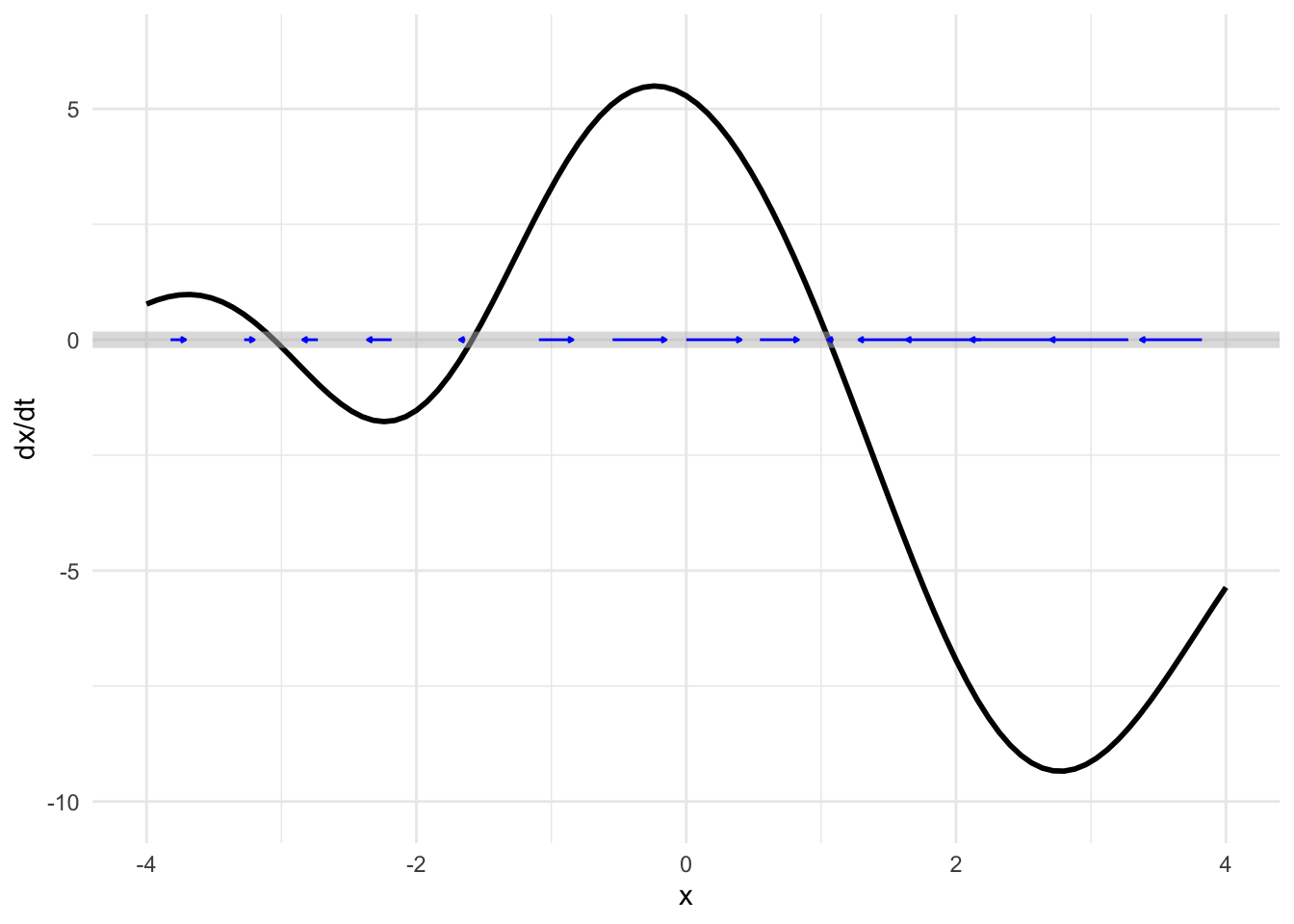
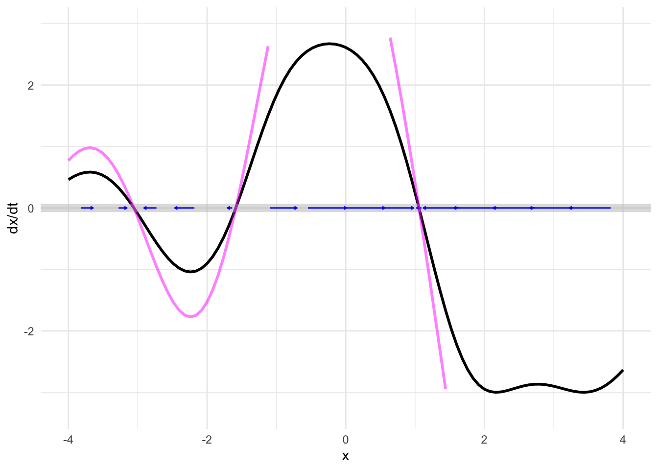
Because the state space can be drawn without using the vertical coordinate of the page, we can use that vertical coordinate to show something else: the dynamical function, as in Figure 46.2.

Figure 46.2: A one-dimensional state space shown with its flow vectors.

The correspondence between the dynamical function and the flow field is easy to see in such a presentation. Where the output of the dynamical is large and positive (say, near $x=0$), the flow is in the positive direction and relatively fast, as shown by a long, right-pointing flow vector. When the output of the dynamical function is negative (around $x=3$, for instance) the flow is in the negative direction: a left pointing arrow.

Near a zero crossing of the dynamical function, the flow arrows are negligibly short: the state velocity is very slow. Indeed, at the zero crossings, the state velocity is exactly zero. Such zero crossings are called fixed points: since the state velocity is zero, the state never moves!

We can see the dynamics near fixed points more closely by zooming in, as in Figure 46.3 which shows two of the system’s fixed points.

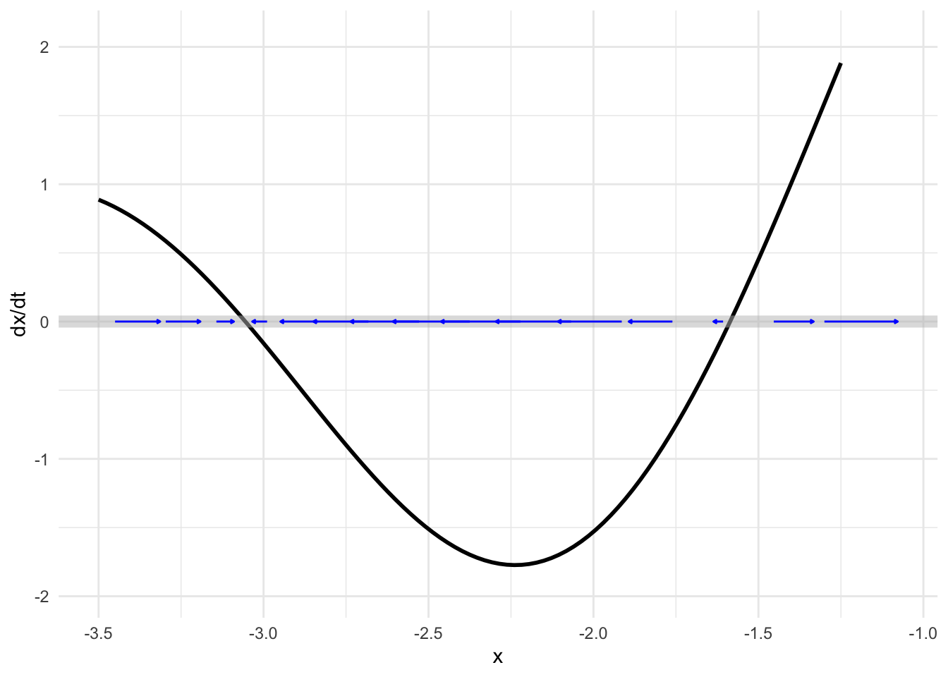
Figure 46.3: Zooming in on the flow for the system shown in Figure 46.2.

Notice in Figure 46.3 that the flow is slower the nearer the state is to the fixed point, but it is only exactly zero at the fixed point.

A calculus technique you will be familiar with from previous Blocks is zooming in a region that we want to examine in detail.

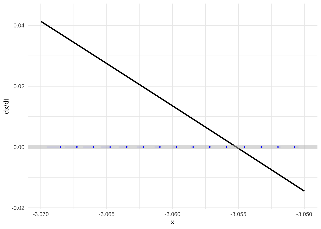
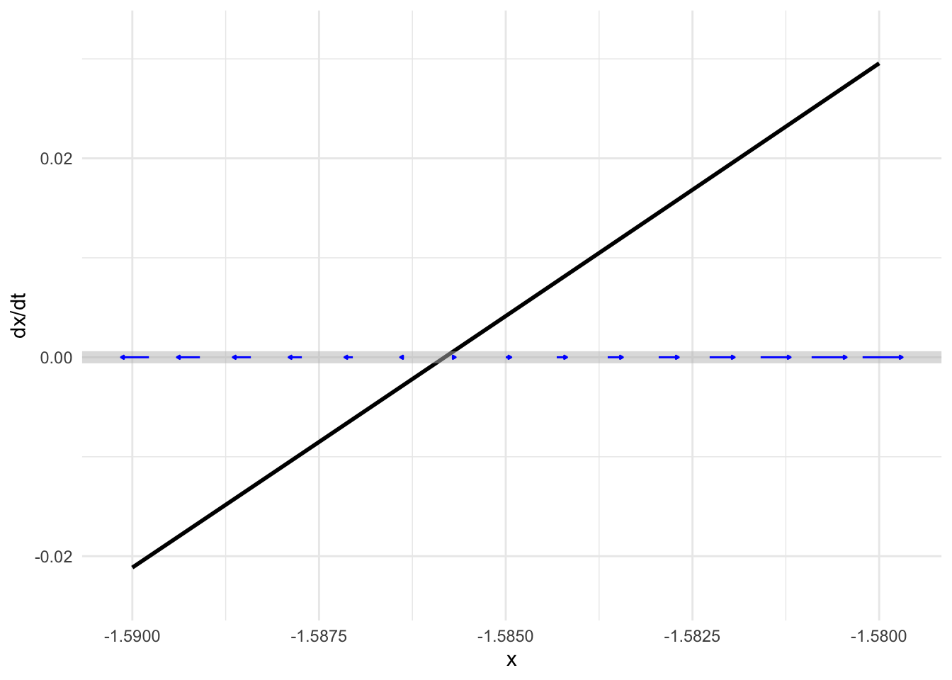
Figure 46.4: Zooming in closely on each of the fixed points seen in Figure 46.3.

The short pieces of the dynamical function shown in Figure 46.4, are, like short pieces of any continuous function: almost exactly straight lines. For the left fixed point, the dynamical function is $f(x) \approx -2.804 (x + 3.055)$ while for the right it is $f(x) \approx 5.065 (x + 1.586)$. In Section @ref(symbolic-solutions-ODE) we found symbolically the solutions for dynamical functions in this form. For $x_0\approx-3.055$ the solution is \[x(t) \approx (x_0 + 3.055)e^{-2.804 t} - 3.055\ ,\] while for $x_0\approx -1.586$ the solution is \[x(t) \approx (x_0 +1.586)\, e^{5.065 t} - 1.586\ .\] There is something fundamentally different about these two solutions. One of them is exponential decay toward the fixed point, while the other grows exponentially away from the fixed point. We call the dynamics near the fixed-point with exponential decay stable and the dynamics near fixed-point with exponential growth unstable.

Tip

Graphics such as Figure 46.2 let you see both the flow and the dynamical functions together in one place.

How about also showing trajectories? Unfortunately, the two-dimensional extent of a computer screen or a piece of paper make it hard to include still more information in an intelligible way. It would be nice to have a third dimension for the display.

Major Austin Davis developed such a display, using time as the third dimension. In the movie below, the state space is shown as a horizontal line, as before. The vertical axis shows the dynamical function as in Figure 46.2. The dynamical function is shown in another way: as the hue and intensity of color, which lets you focus on the activity in the state space. This activity is shown by the moving gray triangles. Each triangle is placed on the phase line to mark an initial condition, then moves right or left according to the dynamics.

46.1 Generic behavior

So long as two dynamical systems have similar fixed points with the same stability, their trajectories will be much the same. For example, our model dynamical function might be different in detail, as in Figure 46.5, and still produce the same behavior.

Figure 46.5: The dynamical function shown in black is a distortion of $f(x)$ from the previous plots. Yet the flow field is practically identical and leads to the same outcomes as $f(x)$ for any initial condition.

So long as two flows have similar fixed points with the same stability, their trajectories will be much the same. Consequently, studying the fixed points without worrying about the details of the dynamics gives a huge amount of information about the system.

For example, Figure 46.6 shows a score of different time series following the solutions from a score of initial conditions. The long-term behaviors for all the time series is similar: they converge to one or another of the stable fixed points.

Figure 46.6: Time series from the differential equation $\partial_t x = f(x)$ starting at many initial conditions. The locations of the three fixed points are marked with horizontal lines. All the solutions convert to one or the other of the two stable fixed points in the system, and depart from the unstable fixed point.

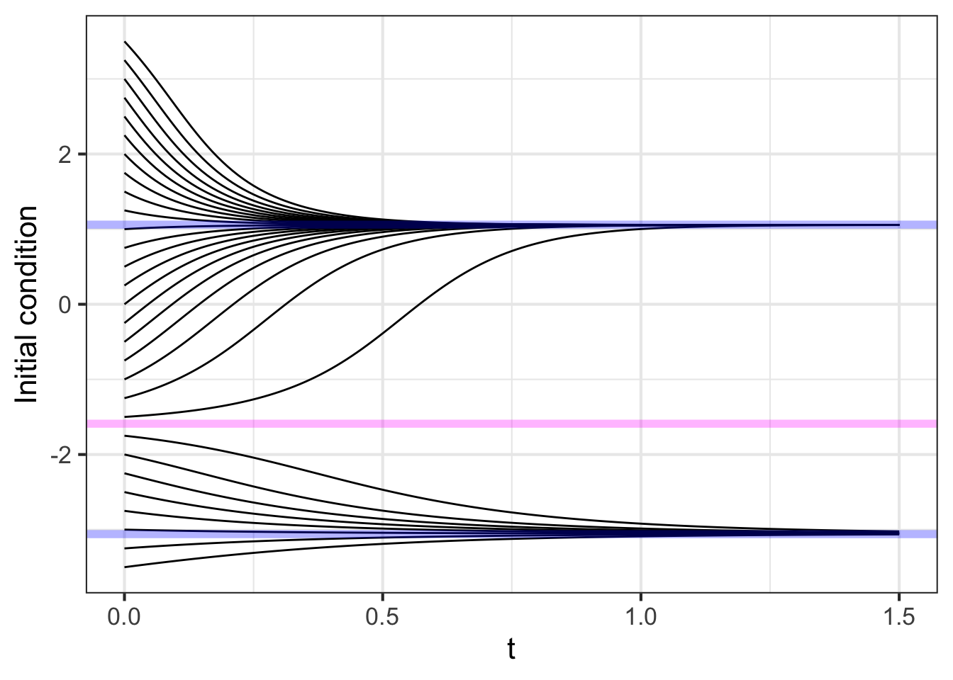
It is worth pointing out a consequence of the mathematics of continuous functions: if a system with a continuous dynamical function has a region of state space with two different fixed points, there must be an unstable fixed point in between them.

46.2 Linearization

You can see in Figure 46.6 that many of the solutions approach their final, equilibrium value in an exponential manner. This is particularly true for the solutions with initial conditions very near the stable fixed points. All these solutions are characterized quantitatively by the parameter $a$ in the exponential solution $A e^{a t}$. (Remember, $a < 0$ when there is exponential decay.)

Quantitative knowledge of $a$ is helpful to understand the time scale of the exponential approach to stable fixed points. We can find a numerical value for $a$ for each fixed point by constructing a linear approximation to the dynamical function near each of the fixed points.

The procedure involves the same principles as introduced in Block 2 for constructing low-order polynomial approximations to functions, but here “low-order” means “first order.”

The analysis is done separately for each of the fixed points, so the first step is to find the fixed points, the values $x^\star$ such that $f(x^\star) = 0$.

Recall from Block 2 the Taylor polynomial approximation to a function $f(x)$ centered on a point $x^\star$: \[f(x) \approx f(x^\star) + \partial_x f(x^\star) \left[x - x^\star\right]\] When $x^\star$ is a fixed point, $f(x^\star) = 0$ so the approximation is simply $f(x) \approx \partial_x f(x^\star) \left[x - x^\star\right]$. Keep in mind that $\partial_x f(x^\star)$ is the derivative function $\partial_x f$ evaluated at the input $x^\star$, so $\partial_x f(x^star)$ is simply a quantity, not a function. Indeed, $\partial_x f(x^star)$ is exactly the quantity $a$ in the exponential solution $e^{a t}$.

This process of constructing the linear approximation $f(x) \approx a \left[x - x^\star\right]$ is called linearization.

Try it! 46.1 Exponential dynamics near fixed points

Consider the first-order differential equation \[\partial_t x = f(x) \equiv r x (x - x/K)\] where $r$ and $K$ are parameters that are greater than zero. Linearizing the nonlinear function $f(x)$ lets us figure out how fast or slow is the exponential growth or decay of the solutions for initial conditions near the fixed points.

There are two fixed points, one at $x_1^\star = 0$ and the other at $x_2^\star = K$. What is the exponential parameter $a$ for each of the fixed points.
The derivative (with respect to $x$) $\partial_x f(x)$ can be found with the product rule from Block 2. It is \[\partial_x f(x) = r\, (1 - x/K) - r\, x\, (1/K)\]
Evaluating $\partial_x f(x)$ at the two fixed points $x_1^\star = 0$ and $x_2^\star = K$ gives

\[\partial_x f(x_1^\star) = r\ \ \ \text{and}\ \ \ \partial_x f(x_2^\star) = -r\] Solutions near $x_1^\star$ will grow exponentially as $e^{r t}$, unstable since $0 < r$. Solutions near $x_2^\star$ will decay toward $x_2^\star$ in an exponential manner as $e^{-r t}$.

Tip

It is critical to distinguish carefully between $x^\star$, which is the location of the fixed point being examined, and $x_0$, which is the initial condition of the state, that is, $x(t=0)$.

Application area 46.1 Retirement savings redux

Let’s return to the model of saving for retirement in Chapter 40: \[\partial_t V = r\, V + M\ .\] The state variable here is named $V$. The dynamical function is \[g(V) = r\, V + M\] where $r$ is the interest rate (say, 3% per year which is $r=0.03$ per year) and $M$ is the monthly contribution. To keep the units consistent, we set the units of $t$ to be years, of $r$ to be 1/years, of $V$ to be dollars and of $M$ to be dollars-per-year. So a monthly contribution of $1000 would come to$M=12000$ dollars-per-year.

Find the amount $V$ that will result from 30 years of savings with an initial condition $V_0 = 0$.

Step i) Find the fixed point. This is a value $V^\star$ such that \[r\, V^\star + M = 0\ \ \ \implies \ \ \ V^\star = -M/r\ .\] Step ii) Find the derivative of the dynamical function evaluated at the fixed point: Since $g(V)$ happens to be a straight-line function, we know the derivative is a constant. So $b = \partial_x g(V^\star) = r$.

Step iii) Translate the state variable into $y = V - V^\star$. The dynamics in terms of $y$ are $\partial_t y = b y$, which has an exponential solution $y = A e^{bt}$.

Step iv) $A$ is the initial condition in terms of $y$. This will be $y_0 = V_0 - V^\star$. Since we stated that $V_0 = 0$ (no savings at the start), $y_0 = -V^\star$ and the solution is \[y(t) = -V^\star e^{bt} = \frac{M}{r} e^{rt}\ .\]

Step v) Translate the solution in step (iv) back into terms of $V(t)$. Since $y(t) = V(t) - V^\star$, this will be $V(t) = y(t) + V^\star$ or, \[V(t) = \frac{M}{r} e^{r t} + V^\star = \frac{M}{r} \left[ e^{r t} - 1\right]\ .\] To get an idea of this retirement plan, that is, $r=3\%$ and $M=12000$ dollars-per-year, let’s see how much you will have after 30 years and 40 years.

V <- makeFun((M/r)*(exp(r*t)-1) ~ t, r=0.03, M=12000)
V(30)
## [1] 583841.2
V(40)
## [1] 928046.8

After 40 years of contributions, your retirement account will have almost one-million dollars.

You could have accomplished the same calculation using integrateODE(), like this:

Soln <- integrateODE(dV ~ r*V + M, V=0, M=12000, r=0.03,  
                     domain(t=0:40))
## Solution containing functions V(t).
Soln$V(30)
## [1] 583841.2
Soln$V(40)
## [1] 928046.8

46.3 Bifurcation

A broad, pressing, social concern goes under the name sustainability. Is it sustainable to burn fossil fuels at steady historical levels, let alone at the increasing rate seen since over the last century? Climate scientists answer resoundingly with a no. Is it sustainable to increase food production to the levels needed for developing economies to approach the sort of consumption seen in rich economies?

Dynamical systems are highly relevant to the questions surrounding sustainability. If the economy is near a stable fixed point, then it is sustainable; the trajectory will bring the state of the economy toward the fixed point. On the other hand, if the economy is near an unstable fixed point, we can expect exponential change.

If such exponential changes are not seen, does that mean we are not near an unstable fixed point? One of the terms used to mark the possibility that a stable system can quickly turn unstable is tipping point, defined as

The point at which a series of small changes or incidents becomes significant enough to cause a larger, more important change. Source: New Oxford American Dictionary

The mathematics of tipping points is not at all the same as exponential growth. Certainly, in exponential growth one sees a relatively slow rate of change increase to a large rate of change, a situation described by journalists as “sky-rocketing” or “explosive” or, literally, “exponential.” As you’ve seen, exponential growth is a phenomenon seen in linear dynamical systems; there is no special point at which the dynamics changes.

There is an area of mathematical theory called catastrophe theory. We will use a famous example to show how catastrophes or tipping points are modeled mathematically.

The example comes from a 1977 article in Nature, one of the world’s most prestigious scientific journals. The article, by Robert May, is entitled “Thresholds and breakpoints in ecosystems with a multiplicity of stable states.” The words “thresholds” and “breakpoints” have not been encountered yet in this book, but “multiplicity of stable states” should bring to mind the sort of dynamics seen in Figure 46.2.

The setting for the catastrophe is an otherwise bucolic scene, livestock grazing on a pasture. A pasture is a kind of factory for producing vegetable biomass; the grazing is the consumption of the biomass produced.

As a model for the production of biomass, denoted $v$ for “vegetation,” we will use \[\partial_t v = r v \left(1 - \frac{v}{K}\right)\] which, as we’ve seen, has an unstable fixed point at $v_1^\star=0$ and a stable fixed point at $v_2^\star=K$. Physically, the fixed point $v_1^\star$ corresponds to a bare field, without any vegetation. It is unstable because any small disturbance in the form of a stray seed landing in the dirt can lead to germination and the rapid growth of vegetation as seeds from the germinated plant spread across the field. Once the field is covered in vegetation, the growth can be exponentially rapid at first but then runs into limited resources: there is only so much sunlight that falls on the field, and the growing vegetation will eventually consume the soil nutrients and water.

This biomass production model corresponds to a sustainable system. Once the biomass level is at $v_2^\star$ it will stay there.

But biomass production is not the only thing going on in the pasture. The grazing animals—let’s imagine they are cows—are consuming the grass. To start very simply, suppose that each cow consumes amount $C$ of biomass each day. If there are $H$ cows, the total consumption is $H C$ per day. This modifies the dynamics to a slightly new form \[\partial_t v = r \,v(1-\frac{v}{K}) - HC\]. The original, ungrazed dynamics are compared with the grazed dynamics in Figure 46.7.

Figure 46.7: Comparing the pasture dynamics for different herd sizes.

With grazing, the net growth of biomass is reduced due to the removal of the consumed biomass by the cows’ consumption. For a moderate herd size, there is still a stable fixed point, but it is at a lower level of biomass than would be seen in the ungrazed field. But if the herd size is too large, the ecosystem completely collapses.

This is an example of a tipping point or catastrophe. For moderate herd sizes, there remains a stable fixed point. A farmer might be tempted to add another cow to the pasture, and that is sustainable: there is still a stable fixed point. Indeed, the movement of the stable fixed point might not even be noticed. But add even one cow too many and the fixed point entirely disappears. Still, herd management can fix the problem; take away the cow that tipped the pasture and the fixed point will return.

Application area 46.2 Cows eat grass

Chapter 16 illustrated the iterative process for building models: using the results of a model to suggest possible improvements in the model. Let’s look again at how cows eat grass.

Missing from the pasture model is a simple idea of how cows eat. If there is very little biomass, the cows cannot continue to eat their fill. Will the reduction in consumption per cow preserve the stable fixed point?

In his Nature article, May modeled the consumption rate by a single cow with the functional form \[C(v) \equiv \frac{\beta v^2}{v_0 - v^2}\] which is graphed for $\beta=0.1$ and $v_0 = 3$ in Figure 46.8

Figure 46.8: Consumption of vegetation by a single cow as a function of the amount available in the pasture.

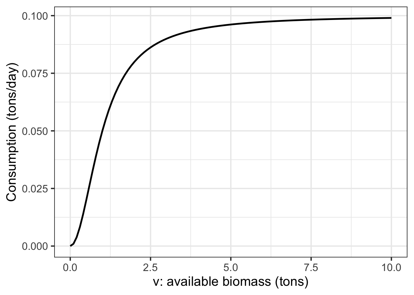
You can recognize this as a form of sigmoid. When the amount of vegetation is very large, a cow will eat her fill. That is the saturation of the sigmoid. For small $v$, the cow needs to hunt around for vegetation tall enough to eat, reducing the consumption steeply.

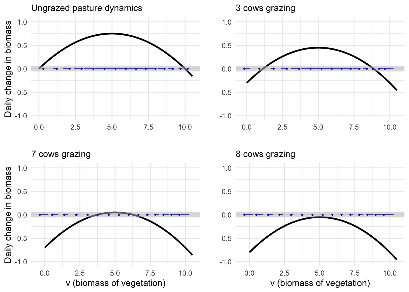
Figure 46.9 modifies the pasture dynamics to incorporate this sigmoid model of consumption.

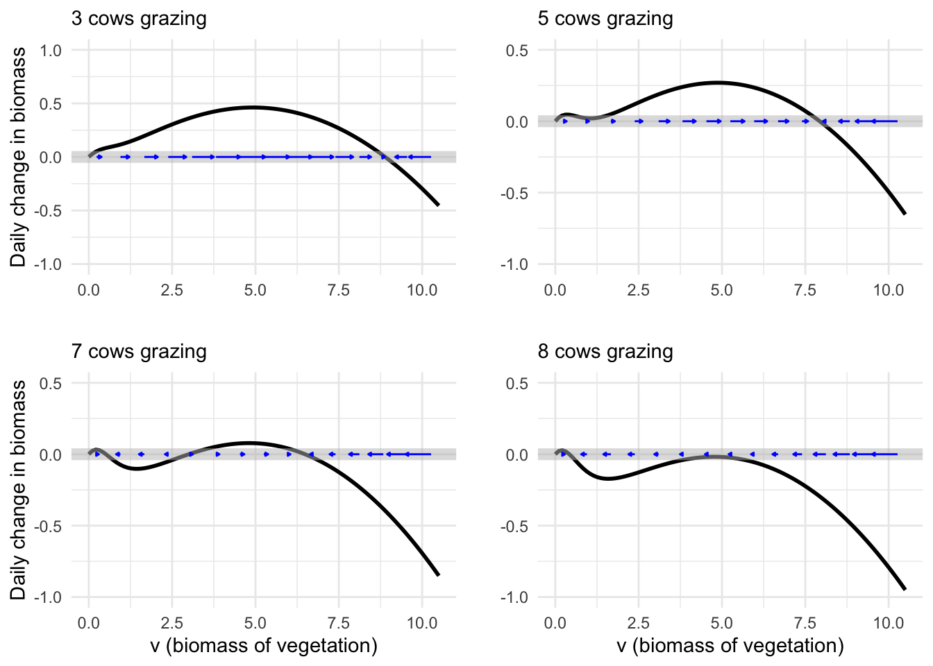
Figure 46.9: Pasture dynamics for a sigmoid consumption function.

We can start the story with 3 cows in the pasture. Vegetation growth is more than sufficient to provide for these cows. You can see this from the stable fixed point at about 9 tons of biomass, which is more than enough to reach saturation of the sigmoid consumption function.

The farmer decides to increase the herd to 5 cows. Nothing much happens. The stable fixed point is at about 8 tons of biomass, entirely adequate to keep the cows well fed in a sustainable manner.

Can the pasture be sustainable with 7 cows? The stable fixed point remains, now at about 6.5 tons at biomass. The cows are still sustainably well fed.

You can see in the 7-cow dynamics a hint of what of what might go wrong. There is a new, unstable fixed point at about 3 tons of biomass. If the pasture ever happened transiently to fall below 3 tons—say due to a summer frost followed by a return to normal weather—the vegetation biomass will head toward the new stable fixed point at 0.5 tons of biomass. At this level, the cows are eating only about one-quarter their normal amount and we can fairly say that the ecosystem has collapsed. But until such a disaster happens, the farmer will see only a sustainable level of biomass with cows well fed.

It is only we, who have a mathematical model of the situation, who can anticipate the potential problems.

Since things are fine with 7 cows in the field, the farmer lets an eighth cow join the herd. That is the tipping point. The happy herd fixed point at 6.5 tons of biomass has disappeared, and the ecosystem collapses, even without a weather disaster.

Removing the eighth cow from the pasture will not fix the situation. With seven or even six cows in the pasture, the system won’t be able to grow out of the stable fixed point with 0.5 tons of biomass. Reducing the herd size to five will remove that 0.5 ton fixed point, but the grass will grow back very slowly; the dynamics give positive growth, but very close to zero.

Avoiding such catastrophes is a major motivation for mathematical modeling.

42 Flows on the line

42.1 Dynamical function and flow

43 raw <- doodle_fun( ~ x, seed=920)

44 Znotes::phase_line(raw(x) - 2 ~ x, bounds(x=-4:4),

45 nix_dyn=TRUE, narrows=25,

46 transform=function(x) x^.75)

46.1 Generic behavior

46.2 Linearization

46.3 Bifurcation