Chapter 14 Simulations
Let’s return to the question of how the choice of model – Y  X or Y X + C is the better one to use for elucidating the effect on Y of an intervention on X. An important tool is simulation, which in this case means generating artificial data using a mathematical mechanism that corresponds to the selected graphical causal model of interest. Because you, the modeler, are generating the simulated data, you know exactly the mechanism underlying it. This lets you try out the different possible models and choose one that most faithfully reproduces the mathematical relationship that generated the data.
Keep in mind, of course, that the simulation does not tell you what is the causal mechanism in the real world. What you find out from the simulation will be applicable to the real world only if the simulation correctly captures the mechanisms for the real world.
NOTE IN DRAFT: Pick up the example in 7.1.
14.1 Building a simulation
For the purpose of illustration, let’s start by building a simulation for a particular graphical causal network:
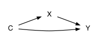
Figure 14.1: The network implemented by the simulations in this section.
In creating simulated data from a graphical causal network, you need to specify, for each variable, what is the function that defines that variable. For example, the variable Y might be defined by the function \(f(C, X) = 2 C - 1.5 X\). Once you’ve defined such a function for every variable, the simulation evaluates that function using the appropriate other variables as input.
In order to make clear which function determines which variable, we’ll use the formula notation, for instance, Y ~ 2 * C - 1.5 * X. This is very much like the formula notation we’ve been using in graphics, statistics, and models, but there are some subtle differences:
In graphics, statistics, and models, the formulas define the response variable and a set of explanatory variables. But in simulations, the formula define an output and a specific mathematical expression that specifies how the output is to be calculated. You always need specific mathematical expressions to create simulated data, whereas in graphing or modeling data you only need to say what are the explanatory variables and what is the response variable.
For defining a simulation of Figure 14.1 we’ll need three functions, one for each of X, Y, and C. Here’s one possibility:
| Network 1 | . |
|---|---|
X ~ 10 * C |
. |
Y ~ 2*X - 4*C |
. |
C ~ 1 |
. |
The odd man out here is C ~ 1. This is saying that C is a function without any inputs. When you evaluate that function, the output is always 10. Admittedly, not a very interesting function.
In running the simulation, you specify how many rows you want in the data frame that will be produced by the simulation. For instance, Table @ref(tab:simulation_1) contains output from Simulation 1 with n = 100 rows.
| C | X | Y |
|---|---|---|
| 1 | 10 | 16 |
| 1 | 10 | 16 |
| 1 | 10 | 16 |
| 1 | 10 | 16 |
| … and so on for 100 rows altogether. |
Table @ref(tab:simulation_1) might be disappointingly simple, but it’s exactly what Simulation 1 calls for. That simulation says that C will always have the value 10. The values of X and Y must also be the same in each row, since they are ultimately based on C. There’s no variability in any of the variables.
To make a simulation that incorporates variability, we need to have a source of variation from one row to the next. Almost always, that variation is provided by a random number generator. Let’s define Simulation 2, making C the output of a random number generator called unif().
| Network 2 | . |
|---|---|
X ~ 10 * C |
. |
Y ~ 2*X - 4*C |
. |
C ~ uniform() |
. |
| C | X | Y |
|---|---|---|
| -0.57 | -5.69 | -9.11 |
| 1.50 | 14.98 | 23.97 |
| -0.46 | -4.64 | -7.42 |
| 0.15 | 1.47 | 2.36 |
| … and so on for 100 rows altogether. |
In networks, variables like C, which have no other variables as inputs, are called exogenous variables. The prefix “exo” means “external” or “exterior”. The root “gene” (like Genesis or gene) means “born.” Exogenous variables arise from outside of the system. In contrast, variables like X and Y, which depend on other variables in the network, are called endogenous: they are inside the system.
Every simulation must have at least one exogenous variable. You have to start somewhere when producing the simulation.
Often, there is more than one exogenous variable. This might be written explicitly as in C ~ uniform() or it might be unnamed as in Network 3, where an endogenous source of variation of written directly in the formulas for X and Y. Note that each time a random generator such as uniform() is used, it generates a different set of random numbers. So the uniform() in the formula for X and that in the formula for Y will give different random numbers.
| Network 3 | . |
|---|---|
X ~ 10 * uniform() |
. |
Y ~ X + uniform() |
. |
| X | Y |
|---|---|
| 11.28 | 12.00 |
| 10.61 | 11.29 |
| -17.11 | -15.62 |
| -12.59 | -11.39 |
| … and so on for 100 rows altogether. |
In the simulations we’ll use throughout this book, you’ll see four different kinds of random number generators:
uniform()which generates numbers equally likely to be anywhere between zero and one. (Or between some other specifiedminandmax.)gaussian()which generates numbers with a bell-shaped distribution.discrete()which generates random levels of a categorical variable.tossup()which generates either one of two possible levels, much like a coin flip.
We’ll use simulations in several places in this book to illustrate when models can give appropriate or misleading results.
14.2 Example: Simulating votes
Consider the following hypothesis regarding spending by political candidate A. Suppose that variable spend is the amount spent on advertising, etc, and that competitive indicates how competitive the election will be, for instance, how popular is the candidate’s opponent. The higher the value of competitive, the lower the proportion of votes for A. But the more A spends, the higher the proportion of votes for A. And the more competitive the election, the more money A will work to raise and spend. We want to simulate a data frame, with one row for each of many elections (e.g. the 435 elections for the US House of Representatives), that will show the relationship between spending and vote outcome. Here’s one possible set of functions implementing the above:
| competitive | spending | proportion |
|---|---|---|
| 0.30 | 9 | 69.5 |
| 0.52 | 27 | 45.9 |
| 0.38 | 15 | 61.2 |
| 0.56 | 32 | 52.0 |
| 0.23 | 5 | 62.0 |
| … and so on for 435 rows altogether. |
competitive ~ uniform(min = 0.2, max = 0.8)spending ~ 100 * competitive^2proportion ~ 70 - 30 * competitive + spending / 20 + gaussian(sd = 5))
Figure 14.2 shows the relationship between spending and vote outcome for n = 435 simulated elections. To look at the graph, you would understandably conclude that higher spending is associated with lower vote percentage. But we know, because it’s written in the formulas used for the simulation, that the opposite is true. An important theme of the rest of this book is how to avoid such paradoxes.

Figure 14.2: The simulation of campaign spending and election results.
14.3 Determinism and randomness
Each of the variables in a simulation mixes, to a greater or lesser extent, two sources of variation:
- A deterministic component that comes from the other variables included in the function. For instance, if the simulation
y ~ 3 + 2 * x - z + 5 * gaussian(), the deterministic component is3 + 2 * x - z. This is called deterministic because the values of the input variables,xandz, completely determine the value of this component ofy. - A random component consisting of the exogenous value of
5 * gaussian(). This is random because (1) it varies and (2) it doesn’t depend on any other variable, that is, it is independent of all the other variables.
The word “random” suggests to many people that the value could be anything at all. This is too simplistic. Every exogenous source used in simulations has an important regularity. The different possible values produced by the source each are assigned a definite probability. This is called a probability distribution. The probability distribution describes which values are more likely than others. Figure 14.3 shows the probability distribution of two endogenous sources commonly used in simulation: gaussian() and uniform().

Figure 14.3: Random values generated by gaussian() and uniform(). The violin plots show the probability distribution of each.
The Gaussian probability distribution is often described as bell shaped. This can be a little hard to see in Figure 14.3; due to the symmetry of the violin depiction of distribution, it looks more like a canoe, or perhaps two bells placed sideways mouth to mouth. Large values (either positive or negative) are sometimes produced by a Gaussian distribution, but they are uncommon.
In contrast, the uniform distribution is box shaped. Any value within the range of the distribution is equally likely: uniform. Values outside this range are impossible.
There are two quantities that describe the random sources used in our simulations: the mean and the variance. The mean, as you might expect, locates the center of the distribution. The variance tells how far, on average, values are from the mean.
Both gaussian() and uniform() are set up to generate values with zero mean. This is not to say that each individual value is zero – from Figure 14.3 you can see that only a handful of values themselves are very close to zero. Instead, it means that the mean of a large enough sample of values will be practically zero.
Similarly, both gaussian() and uniform() are set up to generate values with a variance of 1 (sometimes called “unit variance”). Looking at Figure 14.3 you can see that the spread of values appears similar for the two distributions. Even though the Gaussian reaches further out from the mean, such values have small probability.
Using exogenous sources, like gaussian() or uniform(), with zero mean and unit variance provides a convenient way to compare the sizes of the deterministic and random components of any variable. To illustrate, consider the simple simulation x ~ uniform(), y ~ x + uniform(). The variable x is completely random, since there is no deterministic component (that is, no component that depends on other variables in the simulation). The variable y is a mixture of a deterministic component x and the random component uniform().17
Statisticians use the variance as a preferred measure of the spread of values because variance has an important property. When a variable, say y is the sum of a deterministic component and a random component, the variance of y will exactly equal the variance of the deterministic component plus the variance of the random component.
This additive property of variance provides an unambiguous way to describe how much of the variation is a simulation variable stems from the deterministic component and how much from the random component. For instance in the simulation x ~ uniform(), y ~ x + uniform(), we know that x will have unit variance – that’s the way uniform() works. The variable y has both a deterministic component x and a random component uniform(). The variance of x, as we’ve already seen, is 1. Similarly, the variance of uniform() is 1. So the variance of y will be the variance of x plus the variance of uniform(). In other words, the variance of y is 1 + 1 = 2.
In designing a simulation, you may have a specific notion of what proportion of each variable should be random. (The proportion of variance contributed by the deterministic proportion is called R-squared (\(R^2\)), something we’ll come back to in Chapter 19.) If you want to change the variance of a component, simply multiply it by a contant number (that is, a number that doesn’t vary). After multiplication, the variance will be changed by a factor of the square of the multiplier. Table 14.4 shows some examples.
| System | y ~ x + uniform() | y ~ 3*x + uniform() | y ~ 2x + 5uniform() |
| Determinisitic part of y | x | 3 * x | 2 * x |
| Random part of y | uniform() | uniform() | 5 * uniform() |
| Variance of y | 2 | 10 | 29 |
| Determin. variance | 1 | 9 | 4 |
| Random variance | 1 | 1 | 25 |
| R-squared | 0.500 | 0.900 | 0.143 |
14.4 Inverse simulation
NOTE IN DRAFT: Cornfield’s 1951 calculation
You might wonder why
xis deterministic when it comes to its role iny. Remember, the deterministic component of a variable is that which stems from other variables in the simulation. So far asyis concerned, the origins ofxare unimportant. Also keep in mind thatuniform()is not a particularly set of values but a process for generating values. So the values generated byuniform()inxare unrelated to the values contributed byuniform()in y. It is as ifuniform()is an instruction to take a drink from a river. You and your friend can both drink from the same river, but the water you swallow is distinct from that which your friend imbibes.↩