Chapter 20 Calculating confidence intervals with resampling
Sampling variation is about the changing numerical values of statistics as we look at a set of models constructed from different random samples of a population. At a practical matter, at the point where models are being constructed we no longer have ready access to the population. Instead, we have only the data that have been collected already. We finessed this problem of the inaccessibility of the population by using the data already collected as a stand-in for the population. We take random sub-samples from that population stand-in. Of course, the random sub-samples necessarily had smaller n than the data frame from which they were taken.
There’s a problem, however, with looking at sampling variation using trials with smaller n than the actual data. As you’ve seen, confidence intervals depend systematically with n, their length being proportional to \(1 / \sqrt{n}\). The sampling variation we get from many trials with smaller n than the actual data will result in confidence intervals that are longer than we would have gotten if we could have had access to the actual population for generating the trials. This is important because our reason for looking at sampling variation is to judge how replicable our results are, for instance how to compare our results to another research team’s results with their own data drawn from the population.
One way to fix things is to adjust the confidence intervals we get with small-n subsamples using the general \(1 / \sqrt{n}\) rule. That actually would not be a bad approach so long as small-n is large enough so that the general \(1 / \sqrt{n}\) rule is a good approximation. (A more precise rule is \(1 / \sqrt{n - p}\), where \(p\) is a measure of how complicated the model is. See Chapter @ref(small_data).)
A less complicated way to fix things originates in a simple idea. Let small-n be the same as n. In other words, base each trial on a random sample of n rows drawn from our whole data (which itself has n rows). There’s a glitch in this idea, however. Picking, say, 1000 random rows from a source data frame with 1000 rows results in the sample having exactly the same rows as the source! Consequently, such an approach would give absolutely no variability from one sample to another because every sample would be the same.
I call this a “glitch” rather than a “fatal flaw” or “insurmountable obstacle” because there is a slight modification that will set things right. Instead of using our n-row data as the stand-in for the population, let’s use many copies of the n-row data, producing a population stand-in with many times n rows. Then we can draw sub-samples of size n from the population stand-in without every sub-sample including exactly the same rows as the original. This process is called resampling.
20.1 Duplicate and omitted rows
Since each data set generated by resampling is drawn randomly from many copies of the original data, there is the opportunity for some of the original rows to appear two or more times in the resampled data. And, since there will be n rows in the data produced in a resampling trial, each and every repeat of a row necessitates that another row from the original data not appear in that trial.
It works out that, on average, about 37% of the original rows will not appear in a resampling trial. But since we do many trials to quantify sampling variation, each original row will almost certainly appear in at least one trial.
Similarly, about 37% of the rows in a resampling trial will be duplicates of earlier rows.
Resampling is a viable technique for samples of size, say, 10 and larger. But to illustrate the omissions and duplications that appear in resampling, we’ll use a tiny dataset that will make it easy to see which rows have been omitted.
Table 20.1: A sample of size \(n=4\) from the population.
| name | sex | width | domhand |
|---|---|---|---|
| Eleanor | G | 9.3 | R |
| Danielle | G | 9.3 | R |
| Caroline | G | 8.7 | L |
| Hayley | G | 7.9 | R |
[See enrichment: Omissions in resampling.]
The population stand-in consists of many copies of the sample, as shown in Table 20.2.
Table 20.2: (ref:population-stand-in-cap)
| name | sex | width | domhand |
|---|---|---|---|
| Eleanor | G | 9.3 | R |
| Danielle | G | 9.3 | R |
| Caroline | G | 8.7 | L |
| Hayley | G | 7.9 | R |
| Eleanor | G | 9.3 | R |
| Danielle | G | 9.3 | R |
| Caroline | G | 8.7 | L |
| Hayley | G | 7.9 | R |
| Eleanor | G | 9.3 | R |
| Danielle | G | 9.3 | R |
| … and so on for 16 rows altogether. |
Now, in order to carry out the simulation of many studies as was done to generate Figure 15.2, we are going to create a data table that is like Table (???)(tab:kids-feet-population) in having effectively an infinite number of rows, but is based only on our sample. We can construct such a table by creating many copies of the data table for our sample and laying them all head to tail, as in Table 20.3.
Table 20.3: (ref:kids-feet-many-cap)
| name | sex | width | domhand |
|---|---|---|---|
| Eleanor | G | 9.3 | R |
| Hayley | G | 7.9 | R |
| Caroline | G | 8.7 | L |
| Danielle | G | 9.3 | R |
| Caroline | G | 8.7 | L |
| Hayley | G | 7.9 | R |
| Caroline | G | 8.7 | L |
| Hayley | G | 7.9 | R |
| Eleanor | G | 9.3 | R |
| Hayley | G | 7.9 | R |
| Caroline | G | 8.7 | L |
| Caroline | G | 8.7 | L |
| Danielle | G | 9.3 | R |
| Hayley | G | 7.9 | R |
| Caroline | G | 8.7 | L |
The hypothetical whole-population (Table ??) is only approximated by our repeat-sample-many-times table (Table 20.3). But the approximation is good enough to enable us to compute a confidence interval by repeatedly taking “new” samples from the repeat-sample-many-times table and calculating an effect size from each. The quotes around “new” are meant to signal that the data aren’t really new. This process is called resampling – sampling from a sample. Each of the individual trials is a “resample”. The distribution of effect sizes for many resampling is the resampling distribution. From this distribution, we can calculate a meaningful confidence interval.
Figure 20.1: Four resampling trials in which the effect size width ~ domhand is calculated. Collecting together a large number of such trials produces the resampling distribution, from which a confidence interval on the effect size can be established.

| Resampling trial | Resample | Effect size | ||||||||||||||||||||
|---|---|---|---|---|---|---|---|---|---|---|---|---|---|---|---|---|---|---|---|---|---|---|
| Trial 1 |
|
8.80 | ||||||||||||||||||||
| Trial 2 |
|
8.95 | ||||||||||||||||||||
| Trial 3 |
|
8.80 | ||||||||||||||||||||
| Trial 4 |
|
8.80 |
The process of computing a confidence interval using resampling is called bootstrapping. The word comes from the absurd image of a person lifting himself by pulling on his own boots. This is also the origin of “booting” (or “rebooting”) a computer: a program that starts up a computer so that it can run programs.
20.2 Confidence bands
This picks up on the running time versus age and sex functions in the sampling variability chapter.
I think it’s helpful to display the results from each sampling trial as an individual function, as in Figure 15.3. Sometimes, statisticians prefer to display this sampling variability using a graphical band, called a confidence band, as in Figure 20.2.
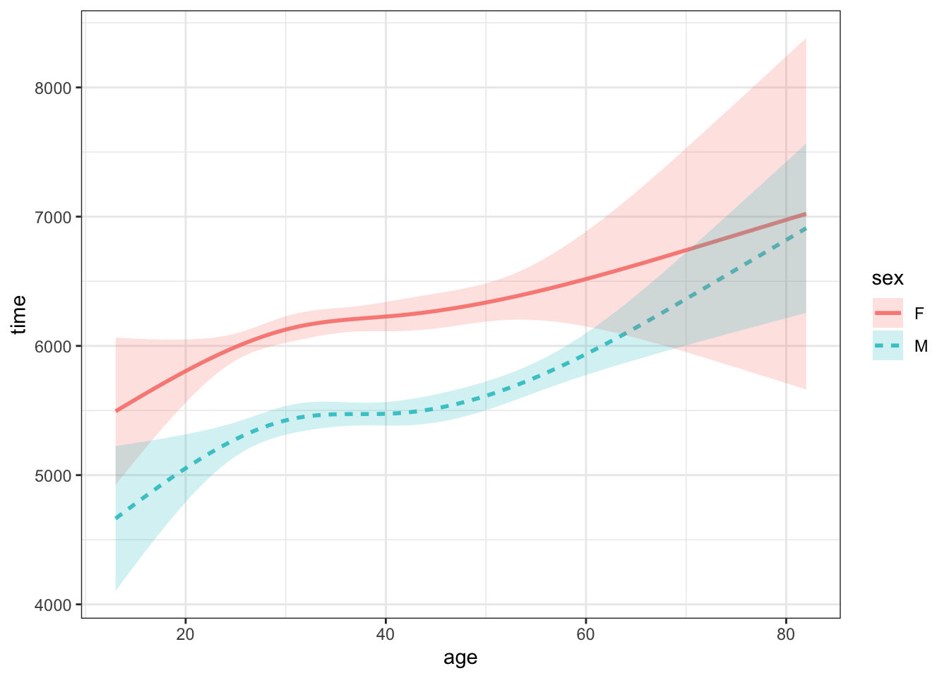
Figure 20.2: Confidence bands showings sampling variation in a function time ~ age + sex trained on a sample of n = 1600 from the ten-mile race data.
20.3 Prediction intervals vs confidence intervals
In Chapter 10 we built a model of the probability of precipitation as a function of air pressure, temperature, wind direction, and wind velocity. (See Figure 10.9.) For convenience, part of that model is reproduced in Figure 20.3.
Figure 20.3: A model of the probability of precipitation conditioned on air pressure, temperature, wind speed, and wind direction. This graph is just two of the panels from 10.9, showing results for a wind speed of 6 mph and wind directions from the north (0 degrees) and south (180 degrees).
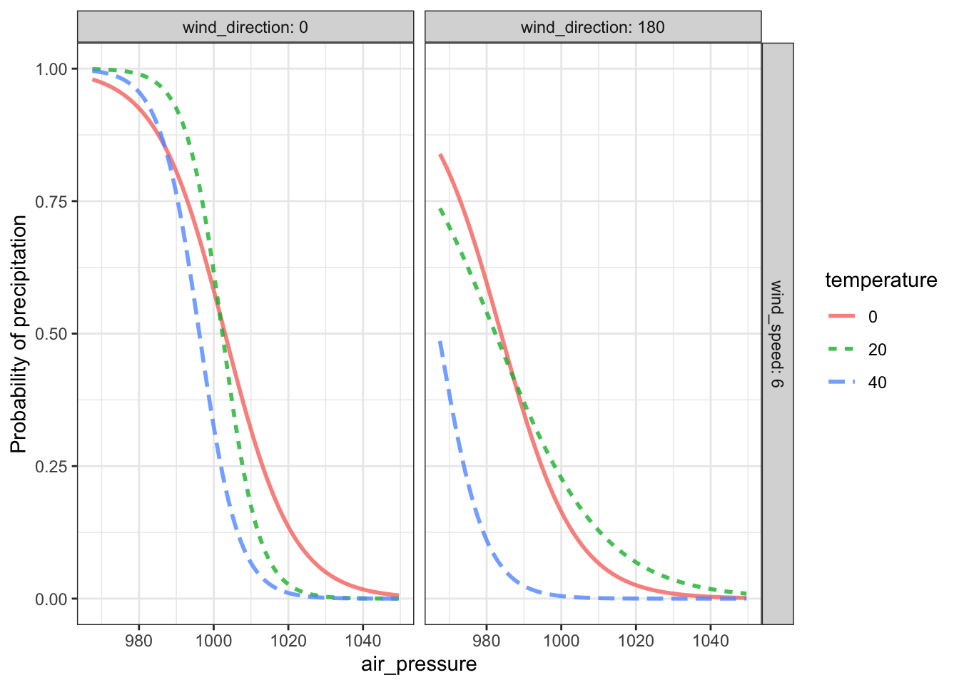
The model shown in Figure 20.3 paints a satisfyingly precise-looking picture of precipitation. When the wind is from the north, the probability of precipitation is pretty much only a function of air pressure and, at low pressure, is almost 100%. When the wind is from the south, the probability is less, especially at 40°F.
Figure 20.4: (ref:rain-confidence-cap)
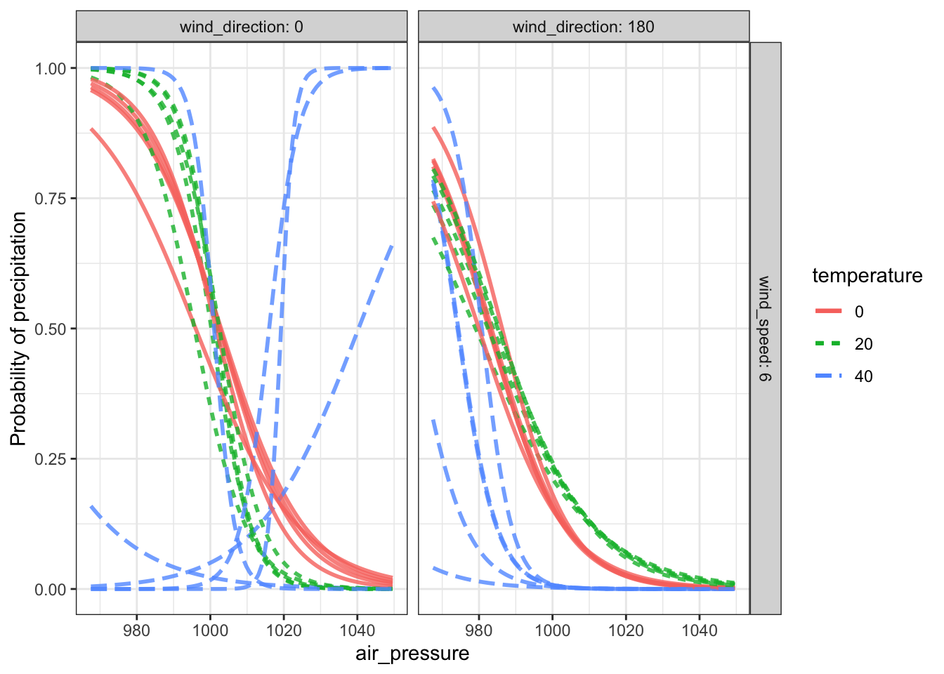
Looking at a few resampling trials tells a somewhat different story. For temperatures of 0 and 20°F, the trials are very consistent with one another. But at 40°F the resampling trials are all over the place, particularly when the wind is from the north (direction 0). It turns out that there is little data when the temperature is around 40°F and the wind is from the north. Confidence in the model output in these conditions is weak.