Chapter 5 Prediction
A prediction is a statement about the as-yet-unknown outcome of an event or situation. The outcome might be whether a patient has cancer, the winner of an upcoming political election, the weather next week, whether a customer will by a product recommended by an online system, or any of a huge variety of other things. Typically, you have some knowledge of the situation, such as the patient’s family history of disease or the prior purchase history of the customer. In statistical prediction, such knowledge is in the form of values for explanatory variables. These values are the inputs to the prediction process. The output of the process is, naturally, the prediction itself, which can be framed as a summary interval of the likely outcomes (for a quantitative response variable) or a listing of the proportion of occurances for each of the levels (for a categorical response variable).
5.1 Stratification and prediction
Stratification provides a simple mechanism for prediction. You pick the response variable, whose value is as yet unknown, for which you will make the prediction. You must already have data on the revealed value of response variable for previous events. Then determine the explanatory variables you want to use to inform the prediction. Of course, these variables should be ones for which you have data for the same previous events for which the response value was revealed. In addition, you meed to know the values of the explanatory variables for the specific case at hand, for which you want to make the prediction. Stratify the response variable by the explanatory variables, identify the stratum that the case at hand falls into, and read out the summary of the response variable for that stratum.
To illustrate, let’s predict the weather! In particular, we’ll make a prediction about whether it will rain in the coming hour and, if it does rain, whether the rain will be light, moderate, or heavy. To keep things simple, the explanatory variable will be whether it has been raining in the hour up to when we make the prediction. Oh … and one other thing. Weather forecasts are always local. The prediction we’ll make will be for a specific place, Saint Paul, Minnesota, where the author lives.
The data we have comes from the US National Oceanographic and Atmospheric Administration (NOAA). There’s a vast amount of data available. If we used the whole collection to make the prediction, we would want to include location as an explanatory variable, setting it to Saint Paul to make the prediction for Saint Paul. But if we’re interested in the Saint Paul stratum, we might as well work with the subset of data just for Saint Paul. This probably seems obvious but it’s worth remembering this rule:
Working with a subset of possible data implicitly amounts to stratifying by the variables that define that subset and picking the particular stratum for that subset.
Later, when we turn to the statistical investigation of causality, it will be important to keep track of the implicit explanatory variables behind our data.
The Saint Paul NOAA data are shown in Table 5.1:
Table 5.1: Hourly weather records from a rainy October night in 1996. The data frame covers the period from July 1996 through July 2018. Quantitative measures of precipitation and air pressure were broken into the discrete levels reported under rain and pressure. The rain_next_hour variable is not part of the original data. The value of rain_next_hour was derived by taking the value for rain_this_hour from the next hour’s data.
| date_time | air_pressure | precip | rain_this_hour | pressure | rain_next_hour |
|---|---|---|---|---|---|
| 1996-10-17 05:53:00 | 998.9 | 0.3 | light | low | heavy |
| 1996-10-17 06:53:00 | 997.1 | 8.4 | heavy | low | heavy |
| 1996-10-17 07:53:00 | 996.8 | 10.7 | heavy | low | light |
| 1996-10-17 08:53:00 | 993.5 | 0.5 | light | low | none |
| 1996-10-17 09:53:00 | 993.2 | 0.0 | none | low | moderate |
| 1996-10-17 10:53:00 | 991.4 | 4.6 | moderate | low | none |
| … and so on for 61,071 rows altogether. |
The original data didn’t include rain_next_hour since that wasn’t known until an hour after each row was recorded. The value of rain_next_hour was added by looking forward in the historical data. The prediction produced by stratifying rain_next_hour ~ rain_this_hour is shown in Table 5.2.
Table 5.2: A stratification of the rain in the next hour by the rain in the current hour. (Values are in percent.) Such a stratification can be used to make a simple prediction.
| none | light | moderate | heavy | |
|---|---|---|---|---|
| none | 97.3 | 49.0 | 27.2 | 30.2 |
| light | 2.4 | 45.3 | 48.3 | 41.1 |
| moderate | 0.2 | 4.4 | 19.1 | 17.1 |
| heavy | 0.1 | 1.3 | 5.5 | 11.6 |
Read Table 5.2 with care. The first column refers to occasions when there has been no rain in the past hour. On such occasions, the next hour is overwhelmingly likely (97.3%) not to have rain either. A heavy rainfall in the next hour is very unlikely: 0.1%. On the other hand, if it has been raining heavily over the past hour, more often than not the next hour will have no rain (30.2%) or light rain (41.1%).
We could choose to use other or additional explanatory variables in the stratification. Some that come to mind include temperature, barometric pressure, and wind direction. And, recognizing that weather patterns shift by month, we might want to stratify as well by month of the year. Going further, we could add to the data measurements made at other NOAA stations in the region. For instance, the town of Minnetonka is about 20 miles west of Saint Paul. Knowing if it is raining now in Minnetonka might be informative about what the next hour has to bring in Saint Paul.
It’s tempting to think that including more and more explanatory variables will always improve the quality of the prediction. One of the important lessons of statistics is that this is not the case. Adding additional explanatory variables might actually worsen the prediction.
When chosing explanatory variables for the purpose of prediction, it helps to be able to measure how good the prediction is, that is, the level of prediction performance. This will be an important theme of the rest of the book. Once we know how to measure prediction performance we can answer questions like, “Is this variable helpful?” or “Would having more data improve the prediction?”
5.2 Prediction of quantitative response variables
The process of predicting the value of a quantitative response variable is very similar to that for categorical response variables. The difference is that we have a choice of available summaries for quantitative variables: point summaries such as the mean or median, interval summaries at various levels, etc. Which ones are best?
An example will help in thinking about the question. Suppose you are thinking about renting a house. You know what the rent will be, but you also have to pay the utilities. It will be helpful to have an estimate of the cost of utilities so that you can work this into your budget. In the real world of rentals, asking how big the monthly utility bill is will produce an answer like this: “A typical month is about $100.” But the landlord – presumably a data-oriented kind of person – has records for the last 20 years or so. The data is broken down by month, and you calculate the mean bill for each month of the year. Your prospective housemate thinks the median will be more informative. Figure 5.1 shows the bill stratified by month, summarizing with both the mean and the median.
Figure 5.1: Utility bills stratified by month and summarized by both the mean and the median. (The data are in SDSdata::Energy_bills.)
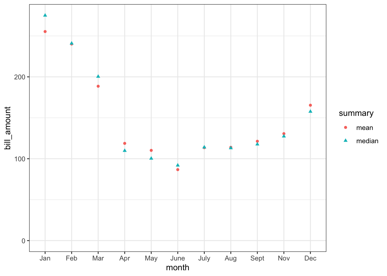
From Figure 5.1, you can see a few things. The claim that “a typical month is about $100” is reasonable, but misleading, since there are three months of the year when the bill is twice that or more. The median bill gives basically the same story as the mean. The crunch time is winter, when you should budget about $200 per month.
But consider now the purpose for the prediction: to budget for the cost of housing. When costs are uncertain, it’s a good practice to take contingencies into account. You don’t want to be in a situation where your housemate can’t pay his share because the amount exceeds his budget. What’s a reasonable contingency amount? You can answer this question, month-by-month, with an interval summary. A 80% interval is arranged to cover all but the lowest and highest 10% of bills. So, if the climate and utility situation don’t change, only about 1 bill in 10 will exceed the upper limit of the 80% summary interval. For comparison, half the bills will be larger than the median.
Figure 5.2: Predictions made in the form of a summary interval can be particularly useful. Here, an 80% summary interval of the monthly bill is shown, as well as a violin, which gives an even more detailed summary.
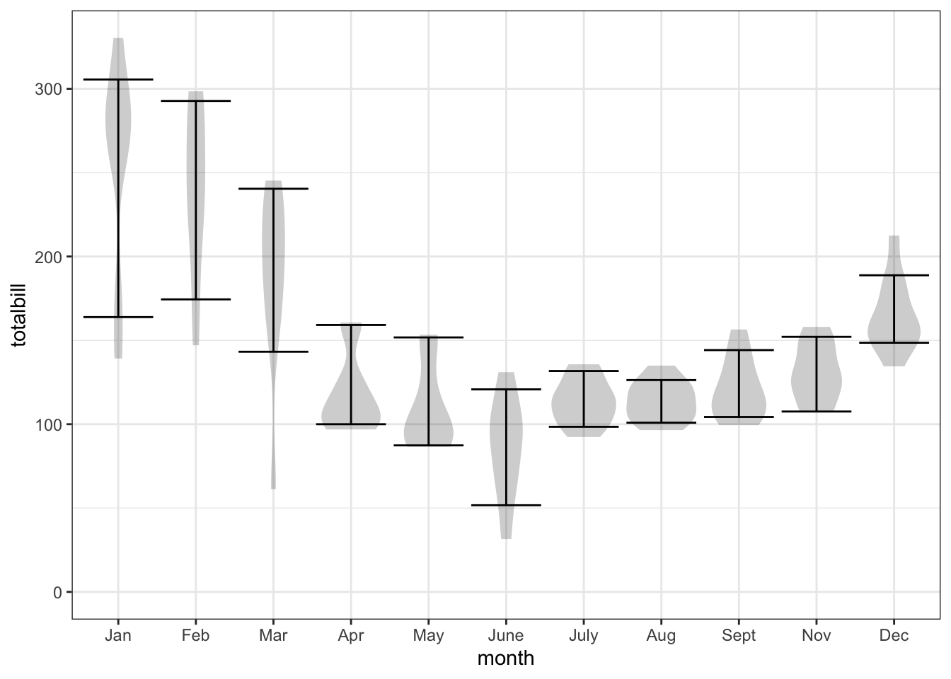
A prediction in the form of an interval gives a much better basis for the decision about how much money to budget each month. Even the lower end of the interval gives some information: “What? You only set aside $100 for the March bill? That’s completely unrealistic!”
A prediction summary in the form of the violins could also be useful, since from the violin you can draw the summary interval at any level: 50%, 80%, 95%. But we don’t yet have the tools needed to make use of this richer format for reporting a prediction.
5.3 Updating predictions
Data doesn’t always come in the form of a complete data table. Sometimes data comes in little bits at a time. In such a situation, it’s nice to have a method for taking the new data into account to update predictions made previously.
Let’s take on a highly controversial matter: Which country will win the next World Cup? A reasonable prediction, at least when one puts aside nationalistic preferences, is the simple statement: Germany will win the next World Cup. You can think of this as a point summary of a prediction. But, although Germany may be the single most likely team to win the Cup, other teams might win instead. Better to report a number for each possible winner, like this:
It’s important to note that the prediction tabulated above does not, and cannot, come entirely from data. I ascribed a 1% chance of winning to Croatia – which has never won the Cup – because in 2018 Croatia came in second place behind France. Surely, securing second place is a good indication of the possibility that a team can win! Similarly, Brazil has won more Cups than any other team but I have put it’s probability at half that of Germany. Why? Because Germany is a more recent winner.
Often, predictions are a matter of opinion. What I think is indisputable in the above prediction is that it mostly says, “I can’t predict exactly who is going to win, just which possibilities are somewhat more likely than others.” Reasonable people can disagree. Someone might put Germany at 40% and someone else at 10%. Neither person will be wrong because, regardless of whether Germany wins or loses, both people have assigned a substantial probability to the eventual outcome.
You might think that such predictions have no point because they don’t point clearly to the eventual outcome. One reason the prediction is useful is that I can use it as a framework for accumulating new information as it comes in. A star player for Germany has been injured? I’ll lower the probability for Germany somewhat and raise the other accordingly. France is starting a phenomenal rookie. Up goes the probability for France (a little) and down with the others.
Another way such predictions are useful is in making decisions. If someone offers me a bet at 1:1 that Germany will win, I will not be inclined to take it since I believe fair odds should be 4:1. (Odds of 1:1 mean that the outcome is seen as equally likely to go either way. In betting, the odds reflect the payout that you will receive. 1:1 odds means that, if you pay $1 to enter into the bet, you will receive $1 + $1 if you win and nothing if you lose. 4:1 odds means that if you pay $1 to enter the bet, you’ll get $4 + $1 if you win.) But if someone offers a bet at 8:1, I will take the bet, especially if I can get someone to accept my 4:1 odds for a second bet, one where I bet against Germany. At 4:1, I’ll pay out $5 on the second bet if Germany wins but collect $9 on the second bet. If Germany loses, my net winnings will be zero. In other words, with such a strategy I’m guaranteed not to lose any money but have some chance of walking away with $4 in winnings.
Predictions that we use as a framework for incorporating new information are called priors, because the prediction exists before the information is known. Once we’ve revised the prediction, it’s called a posterior because that’s after the information is known. In typical use, as each bit of new information comes in, we take the prior and revise it into a posterior. Then, we use the posterior as the new prior for information that might come in later.
5.4 Predictions about interventions: causality
Sometimes a prediction is made in order to anticipate the change that will happen in response to some intervention. For example, suppose I propose to turn down the winter thermostat by 4°F in order to save money. How much money will I save?
To make an informative prediction, I need to be careful to use explanatory variables that include the intervention, and to take care to anticipate how the intervention will cause changes in other influences. Traditionally, statistics students have been told to avoid making any statements that involve causation unless drawing on a randomized experiment which looks at the outcome both with and without the intervention being made. But often you need to make a decision about an intervention without the opportunity or even the possibility of performing an experiment. Such decisions are often best guided by making predictions from stratifications that involve carefully selected explanatory variables that reflect how the system is believed to work. This important topic of causal reasoning will be discussed in more detail in later chapters.
5.5 Exercises
- Miscellaneous taken from drafts of this chapter: shark-bit-spoon
Compare rain prediction when stratifying with time and air pressure or time and wind direction or including month.
Compare prediction knowing the current rain status to prediction just knowing the month.
Survival on the titanic.
5.6 Exercises
Problem 1: You are a bus dispatcher in New York City. The Department of Education bus logistics office has called to say that a school bus has broken down and the students need to be offloaded onto a functioning bus to take them to school. Unfortunately, the DOE officer didn’t tell you how many students are on the bus. You need to make a quick prediction in order to decide what kind and how many busses you will need for the pickup.
You go to the NYC OpenData site bus breakdown page to get the historical data on how many students are on the bus. There are more than 200,000 bus events listed, each one of them including the number of students. You make a jitter/violin plot of the number of students on each of the 200,000 busses.
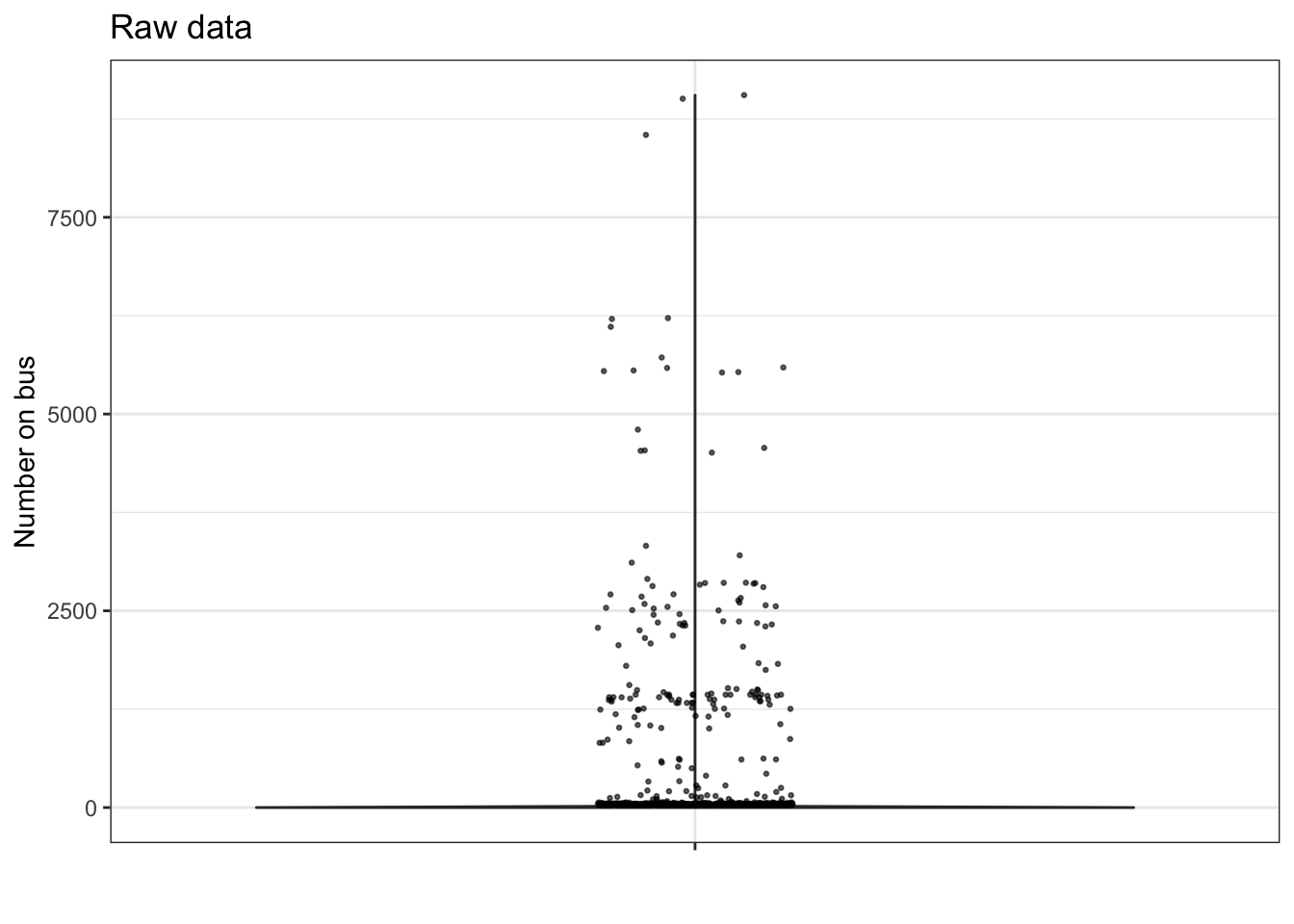
- The violin plot looks like an upside-down T. Explain what’s going on. (Hint: How many students fit on a school bus?)
One of the ways of handling outliers is to delete them from the data. A softer way is to trim the outliers, giving them a value that is distinct but not so far from the mass of values. The figure below shows a violin plot where any record where the number of students is greater than 20 is trimmed to 21.
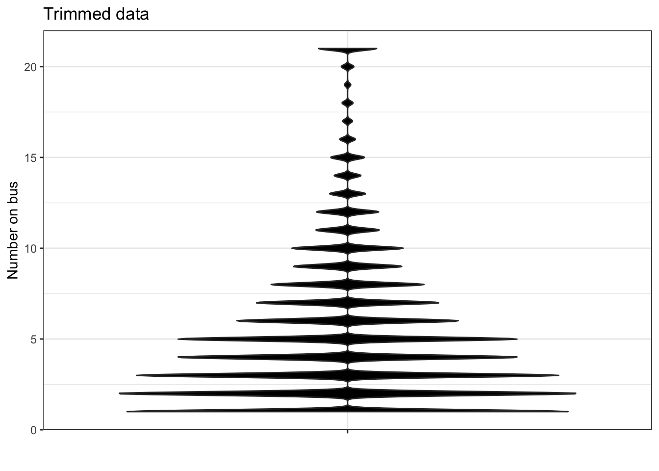
If you sent a small school bus (capacity 14), what fraction of the time would you be able to handle all the students on the school bus?
If you sent one 14-passenger school bus with another on stand-by (just in case the first bus doesn’t have sufficient capacity), what fraction of the time could you handle all the students?
Notice that the violin plot is jagged. Explain why.
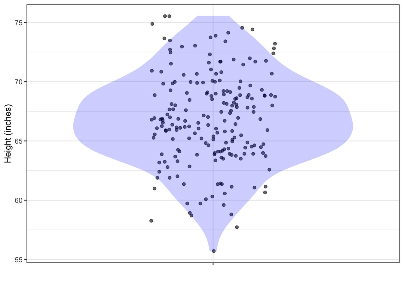
Problem 2: At a very large ballroom dance class, you are to be teamed up with a randomly selected partner. There are 200 potential partners. The figure below shows their heights.
From the data plotted, calculate a 95% prediction interval on the height of your eventual partner. (Hint: You can do this by counting.)
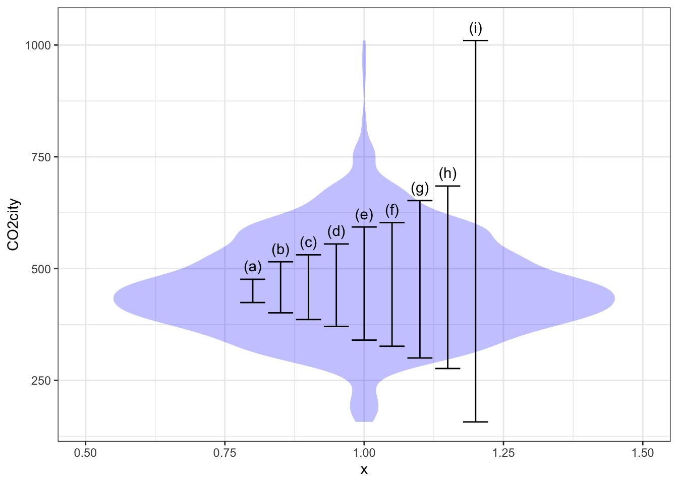
Problem 3: Calculation of a 95% coverage interval (or any other percent level interval) is straightforward with the right software. To illustrate, consider the efficiency of cars and light trucks in terms of CO_2 emissions per mile driven. We’ll use the CO2city variable in the SDSdata::MPG data frame. The basic calculation using the mosaic package is:
##     lower   upper
## 1 276.475 684.525
The following figure shows a violin plot of CO2city which has been annotated with various coverage intervals. Use the calculation above to identify which of the intervals corresponds to which coverage level.
- 50% coverage interval
- 75% coverage interval
- 90% coverage interval
- 100% coverage interval
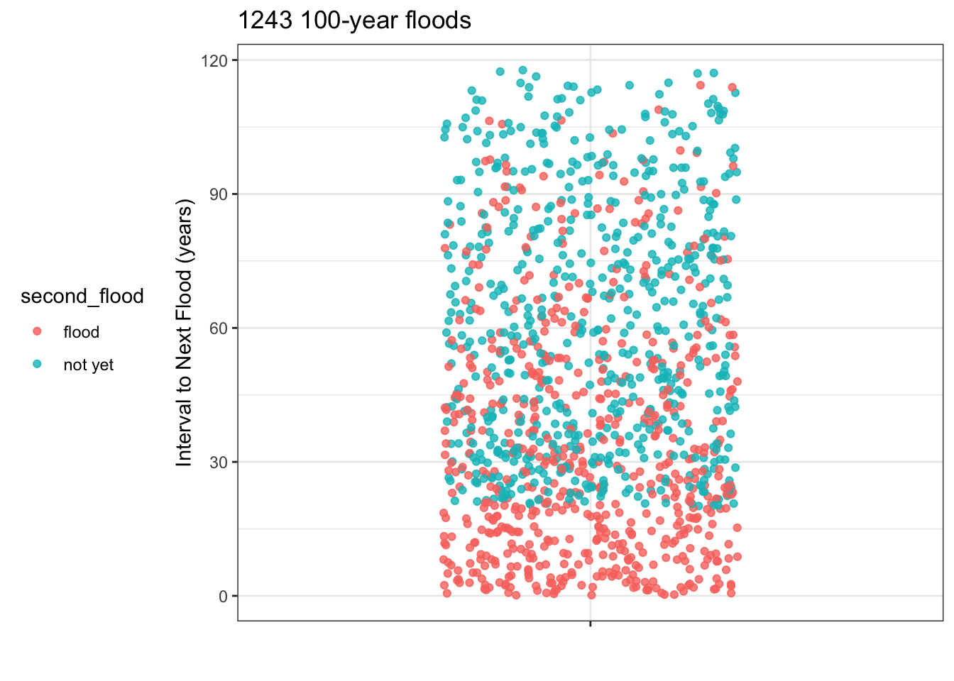
Problem 4: The town where you live has just gone through a so-called 100-year rain storm, which caused flooding of the town’s sewage treatment plant and consequent general ickiness. The city council is holding a meeting to discuss install flood barriers around the sewage treatment plant. The are trying to decide how urgent it is to undertake this expensive project. When will the next 100-year storm occur.
To address the question, the city council has enlisted you, the town’s most famous data scientist, to do some research to find the soonest that a 100-year flood can re-occcur.
You look at the historical weather records for towns that had a 100-year flood at least 20 years ago. The records start in 1900 and you found 1243 towns with a 100-year flood that happened 20 or more years ago. The plot shows, for all the towns that had a 100-year flood at least 20 years ago, how long it was until the next flood occurred. Those town for which no second flood occurred are shown in a different color.
You explain to the city council what a 95% prediction interval is and that you will put your prediction in the form of a probability of 2.5% that the flood will occur sooner than the date you give. You show them how to count dots on a jitter plot to find the 2.5% level.
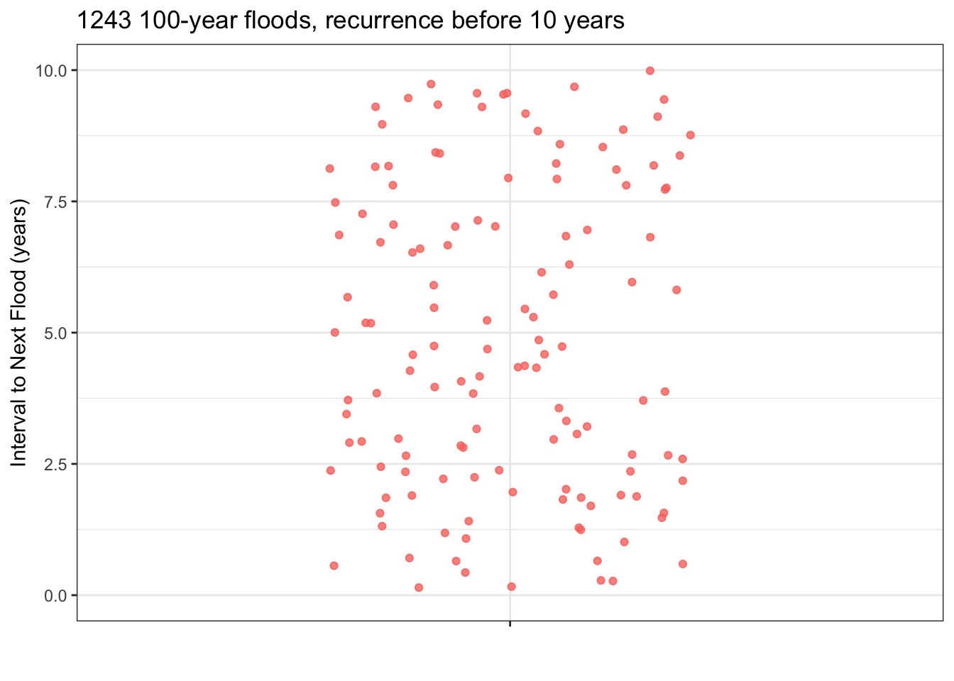
Since the town council is thinking of making the wall-building investment in the next 10 years, you also have provided a zoomed-in plot showing just the floods where the interval to the next flood was less than ten years.
- You have n = 1243 floods in your database. How many is 2.5% of 1243?
- Using the zoomed-in plot, starting at the bottom count the number of floods you calculated in part (a). A line drawn where the counting stops is the location of the bottom of the 95% coverage interval. Where is the bottom of the 95% interval.
- A council member proposes that the town act soon enough so that there is a 99% chance that the next 100-year flood will not occur before the work is finished. It will take 1 year to finish the work, once it is started. According to your data, when should the town start work?
- A council member has a question. “Judging from the graph on the left, are you saying that the next 100-year flood must come sometime within the next 120 years?” No, that’s not how the graph shold be read. Explain why. -a- Since the records only start in 1900, the longest possible interval can be 120 years, that is, from about 2020 to 1900. About half of the dots in the plot reflect towns that haven’t yet had a recurrence 100-year flood. Those could happen at any time, and presumably many of them will happen after an interval of, say, 150 years or even longer.
Problem 5: There are two equivalent ways of of describing an interval numerically that are widely used:
- Specify the lower and upper endpoints of the interval, e.g. 7 to 13.
- Specify the center and half-width of the interval, e.g. 10 ± 3, which is just the same as 7 to 13.
Complete the following table to show the equivalences between the two notations.
Proble 6: You’ve been told that Jenny is in an elementary school that covers grade K through 6. Predict how old is Jenny.
- Put your prediction in the format of assigning a probability to each of the possible outcomes, as listes below. Remember that the sum of your probabilities should be 1. (You don’t have to give too much thought to the details. Anything reasonable will do.)
Age         | 3 or under | 4 | 5 | 6 | 7 | 8 | 9 | 10 | 11 | 12  | 13 | 14 | 15+
------------|------------|---|---|---|---|---|---|----|----|-----|----|----|-----
probability | | | | | | | | | | | | |- Translate your set of probabilities to a 95% prediction interval.