Chapter 19 Partitioning variance

19.1 Why partition?

To put the interest in partitioning in context, consider that the development of statistics as a field was strongly motivated by genetics. Human and agricultural experience over millenia made it clear that offspring inherit to some extent the traits of their parents. In 1859, Charles Darwin introduced his theory that the natural selection of heritable traits drives the origin and evolution of species. But there was very little understanding of what was the mechanism of heritability and almost no notion of how to quantify “to some extent.”

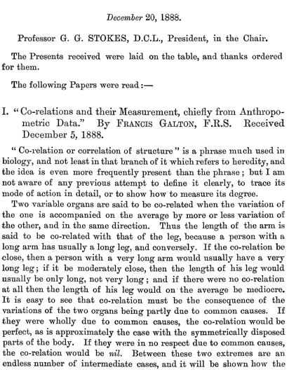
In 1888, Darwin’s cousin, Francis Galton, published the first description of how to measure the “co-relations” between somehow related but variable “organs.” Nowadays, we speak of “correlations” between “variables,” but in these early days of statistics “variable” had not yet become a noun. The biological motivation of Galton’s work is evident from that initial publication, part of which is shown in Figure 19.1.

Biology was at the core of the development of statistics in the late 19th and early 20th century. For instance, the earliest research journal in statistics was (and still is) named Biometrika. Ronald Fisher, the leading figure in statistics in the early 20th century, worked at an agricultural research station from 1919 to 1933, then became chair of the department of eugenics at University College London (1933-1939), then was chair of genetics at the University of Cambridge (1940-1956).1616 In the late 1950s, Fisher, a lifelong smoker, famously attributed lung cancer to genetic factors rather than to smoking. Ironically, he died in 1962 from colon cancer, which, like lung cancer, is caused by smoking.

Consider the equation \[y_i = f(x_i) + \epsilon_i\] in the context of heritability. Suppose \(y_i\) is some observable biological trait, such as height, in person \(i\). Imagine that \(x_i\) is that same or a related trait in the parents of person \(i\). Through some mechanism, unknown in 1888, the parent’s traits are passed along to the child. Even without being able to describe the mechanism, we can give it a name: \(f( )\). And, of course, the trait in person \(i\) is shaped by influences other than heritability, for instance, health, nutrition, and so on. Let’s use \(\epsilon_i\) as the label for these non-heritable influences acting on person \(i\).

While it would be nice to know the details of \(f(x_i)\), that’s a lot to hope for. Instead, Galton asked how much of \(y_i\) can be attributed to \(x_i\) and how much should be attributed to the non-heritable traits \(\epsilon_i\). We often call this question the matter of “nature versus nuture.” And you will encounter claims such as, “addiction is due 50 percent to genetic predisposition and 50 percent to poor coping skills,”1717 https://www.addictionsandrecovery.org/is-addiction-a-disease.htm or “genetic factors underlie about 50 percent of the difference in intelligence among individuals”1818 https://ghr.nlm.nih.gov/primer/traits/intelligence, or “60 to 80 percent of the difference in height between individuals is determined by genetic factors, whereas 20 to 40 percent can be attributed to environmental effects, mainly nutrition” ^https://www.scientificamerican.com/article/how-much-of-human-height/], or “Human family studies have indicated that a modest amount of the overall variation in adult lifespan (approximately 20-30%) is accounted for by genetic factors”1919 https://www.ncbi.nlm.nih.gov/pubmed/16463022.

19.2 Quantifying variability

There are many ways to quantify variability in a numerical variable, for instance the length of the 95% coverage interval. The conventional or “standard” measure of variation, adopted early in the history of statistics, is called the standard deviation. As a rule of thumb, the standard deviation is about one-quarter the length of the 95% coverage interval. Another important way to quantify variability, the variance, which is simply the square of the standard deviation.2020 The word “variance” was introduced by Ronald Fisher in his 1918 paper “The correlation between relatives on the supposition of Mendelian inheritance”. See Charlesworth and Edwards (2018).

To illustrate, consider the Scottish hill racing data. Table 19.1 shows the winning time, distance, climb, and sex. Also shown is the output of a model function time ~ distance + climb + sex Finally, for each row, the model error is given.

Table 19.1: The explanatory and response variables along with the model output and model error for the Scottish hill race data modeled as time ~ distance + climb + sex.

distance	climb	sex	time	model_output	model_error
6	240	M	1630	1286	344
6	240	M	1655	1286	369
6	240	W	2391	2077	314
6	240	W	2351	2077	274
14	660	M	4151	4411	-260
14	660	M	3975	4411	-436
… and so on for 2,224 rows altogether.

Our goal is to find a way to partition the variation in the response variable (time) by the model output and the model error. In other words, we want a way to measure variation that produces this relationship:

\[\mbox{variation in response} = \mbox{variation in model output} + \mbox{variation in model error}\]

To this end, let’s look at several measures of variation and see which, if any, follow the desired relationship.

Table 19.2: Various ways of measuring the spread of the quantities in Table 19.1.

quantity	coverage_lower	coverage_upper	length_coverage	std_dev	variance
time	952	12715	11763	3124	9,759,500
model_output	496	12207	11711	3026	9,158,100
model_error	-1200	1728	2928	775	601,400

You can see from Table 19.2 that the length of the 95% coverage interval does not satisfy the partitioning equation simply because 11763 \(\neq\) 11711 + 2928. Similarly, the standard deviation, which is roughly one-quarter the length of the coverage interval does not achieve the partitioning since 3124 \(\neq\) 3026 + 775. In contrast, the variance does satisfy the partitioning equation: 9,759,500 = 9,158,100 + 601,400.

Don’t be too surprised about the need to square the standard deviation in order to partition the variability. This same phenomenon, for the same mathematical reasons, appears in the familiar mathematics of a right triangle with sides of length \(a\) and \(b\) and hypotenuse of length \(c\):

\[a + b \neq c \ \ \mbox{but }\ \ a^2 + b^2 = c^2\]

19.3 R-squared

One widely used statistic to describe a model involves comparing the variance of the model output to the total variance (that is, the variance of the response variable) with a ratio. This ratio, called R-squared (or \(R^2\) or even the awkward term coefficient of determination.) is taken as describing what fraction of the total variance is accounted for by the explanatory variables. This fraction can range between 0% and 100%.

For the model time ~ distance + climb + sex trained on the Scottish hill race data, the total variance (see Table 19.2) is 9,759,500 square-seconds. The variance of the model output is 9,158,100 square seconds. Consequently the \(R^2\) is \(\frac{\mbox{9,158,100}}{\mbox{9,759,500}} =\) 0.94. We would thus be justified in saying that climb, distance, and sex account for 94% of the variation in winning time.

What accounts for the other 6%? To our model time ~ distance + climb + sex that 6% is just random variation. If we were to look more closely, we might find that the weather, the rockiness or slipperiness of the course, etc. also account for some of that 6%.

A common misconception is to believe that there is some threshold for R-squared that distinguishes between a “good” model and a poor model.2121 Note in DRAFT to instructors: This mythical threshold is often said to be around 15%. I suspect the origins of this misconception lie in a rule of thumb for analyzing experimental data when you have about two-dozen subjects. In this situation, an R-squared of 15% is the smallest you can have before there is any reason to think that the experimental treatment is at all related to the response. Another example of confusing statistical “significance” with substance. This is nonsense. Whether or not a model is good or bad depends on the model’s serving the purpose for which it was built. The \(R^2\) statistic addresses a particular abstract question – how much of the variation is explained by the model – but this is rarely the question that a model is built to answer. For most purposes, an effect size is a better way of describing the relationship between two variables. See Chapter @ref(effect_size).

19.4 The correlation coefficient

Generations of statistics students have been taught to quantify the relationship between two quantitative variables using the correlation coefficient. This is a number, designated r (“little-r”), that ranges between -1 and 1 and offers a very limited description of the relationship.

The correlation coefficient has an honorable historical priority: it came first among modeling techniques. Other than this, it has no fundamental significance to modeling and offers a very limited description of the relationship between two variables.

A good way to think about the correlation coefficient is in terms of a prediction model. As described in the previous section, \(R^2\) is one way of quantifying the performance of a model. The correlation coefficient is merely the square-root of \(R^2\).

So why not write the correlation coefficient as upper-case \(R\) instead of lower-case \(r\). The reason has to do with the restricted set of models to which the concept of \(r\) applies.

• The model must involve a quantitative response variable and a single quantitative explanatory variable.
• The shape of the model must be a simple straight line; no curvature allowed.

One more thing about the correlation coefficient. In taking a square root of \(R^2\), you have a choice between a positive or a negative branch. For instance, the square root of 0.25 is either -0.5 or +0.5. For the correlation coefficient, the sign will be that of the slope of the straight-line model.

In writing this book, I was tempted to leave \(r\) out entirely because little-r is of little use in data science.

19.5 Analysis of variance

We now have a quantity to measure variability, the variance (the square of the standard deviation), that allows us to partition variability in a response variable into components: the component accounted for by the explanatory variables and the component that is left over, that is, the component associated with the model error, \(\epsilon\).

The statistics term analysis of variance refers exactly to this sort of partitioning of variability. The word “analysis” means “to take apart.”

One way to use analysis of variance splits up the “credit” each explanatory variable deserves in accounting for the response variable. Let’s illustrate this using three explanatory variables, distance, climb, and runner’s sex in modeling the winning times in Scottish hill races.

The strategy is to build a series of nested models. In our example, the models will be:

1. model output is constant – the no-input model
2. time ~ distance
3. time ~ distance + climb
4. time ~ distance + climb + sex

Notice that model (4) includes all the explanatory variables in model (3), and model (3) includes all the explanatory variables in model (3). That’s nesting.

Table 19.3 shows how the partitioning of variability into a component associated with the model and a component associated with the error \(\epsilon\).

Table 19.3: The partitioning of variance by a series of four nested models.

model	variance_of_model_output	variance_of_model_error
no input	0	9,759,503
time ~ distance	8,342,237	1,417,266
time ~ distance + climb	9,001,456	758,047
time ~ distance + climb + sex	9,158,149	601,355

Referring to Table 19.3 note that the total variance of the time variable is about 9,759,000 square-seconds, and that, for every model, the variances of the model output and of the model error sum to that total. Also, note that as one moves from one model to the next, the variance of the model output goes up. For instance, the variance for time ~ distance is 8,342,000 square-seconds while time ~ distance + climb has a model output variance of 9,001,000 square seconds. The difference between these, 9,001,000 - 8,342,000 = 658,000, is the amount that can be attributed to the added explanatory variable, climb.

For generations, analysis of variance has been used to test whether a proposed explanatory variable is worthwhile to include in a model. The theory behind this test will be presented in Chapter 21. But for this purpose, there’s little reason to prefer analysis of variance to another method, cross validation. (See Chapter 18.)

Traditionally, in the years before electronic computers became readily available, analysis of variance was presented as a set of formulas involving sums of squares, “grand means”, and “groupwise means.” These formulas accomplished two distinct processes at the same time: training a model and evaluating the change in model output variance from one nested model to another. In this book, with the aid of computers, we treat those processes separately: training a model versus calculating the model output variance.

19.6 Example: Distance, climb, or sex?

The analysis of variance in Table 19.3 suggests that the climb variable contributes marginally to the model output variance: it adds 658,000 square-seconds compared to distance which adds 8,342,000 square-seconds. The sex variable adds even less.

To some extent, the results of analysis of variance depend on the order in which the models are specified. Table 19.4 shows a different order of variables, with sex coming first, climb second, and distance third.

Table 19.4: An analysis of variance for the same model time ~ distance + climb + sex considered in Table 19.3, but with the variables considered in a different order.

model	variance_of_model_output	variance_of_model_error
no input	0	9,759,503
time ~ sex	161,332	9,598,172
time ~ sex + climb	7,624,139	2,135,364
time ~ sex + climb + distance	9,158,149	601,355

With this alternative ordering of variables, we see that sex continues to contribute only a small amount to the variance of model output, while climb is the major contributor. This inconsistency or ambiguity is not so much about analysis of variance but about the ambiguities inherent in attributing “credit” to one variable or another. As it happens, distance and climb are closely related, with longer races tending to have more climb. Thus, distance and climb share information about the winning time. Credit for that shared information can be attributed to either variable.

One of the main applications of analysis of variance is the study of experimental data in which the experiment has been designed in a way to make the various explanatory variables unrelated to one another. Doing this, for example, is the motivation behind randomizing the treatment in experiments, which eliminates any systematic relationship between the treatment and covariates.

References

Charlesworth, Brian, and Anthony W.F. Edwards. 2018. “A Century of Variance.” Significance 15 (4): 21–25.