Chapter 13 Effect size
(ref:chapter-effect_size) Chapter 13
In the previous chapter we looked at \(R^2\), an abstract measure of the relationship between a set of explanatory variables and a response variable. This chapter introduces a simpler and more concrete way of describing relationships: effect size.
As you know, a model prediction function takes inputs and produces an output. With \(R^2\), you’re looking at the overall spread of the inputs from row to row in the testing data and the consequent spread in the model outputs compared to the spread of the response variable. An effect size is different, it doesn’t depend on the spread in the testing data. Instead, an effect size quantifies how a change in an input variable leads to a change in the model value.
Some examples:
A medicine is intended to reduce the probability of flare-up of a disease. An effect size for flare-up probability versus dose describes how much decrease in probability is associated with an increase in the dose of the medicine.
The reading level of primary-school graduates depends on many factors, including for instance the availability of funding for teacher salaries, school maintenance, textbooks, parental involvement, and (perhaps) class size. An effect size of reading level – say measured as grade level – versus salary funding tells how changing salary corresponds to an eventual change in reading level. There will also be an effect size for reading level as a function of class size: how much the reading level of graduates will change if the class size is increased. There will also be effect sizes for reading level versus each of other the explanatory variables.
The extent of climate change depends on how much carbon dioxide (\(\mbox{CO}_2\)), methane, and other greenhouse gasses are emitted into the atmosphere. Measuring climate change by global average temperature, the effect size of climate size versus \(\mbox{CO}_2\) will be in the form of degrees warming per gigaton of \(\mbox{CO}_2\).
13.1 Change in input, change in output
The basic technique for calculating an effect size is extremely simple … once you have constructed an appropriate predictive model.
Imagine a debate between Amelia and Jack, running friends who live in Dundee, Scotland. Which is harder: a hill race that’s longer by 1 km or a race that involves an extra 50 m of climb?
Consulting the records for hill races, the friends construct the model shown in Figure 13.1: time ~ distance + climb + sex. Using the model, they can simulate the effect of adding 1 km or adding 50 m to a race and see how the winning time changes.
Figure 13.1: A model of winning time in the Scottish hill races: time ~ distance + climb + sex.
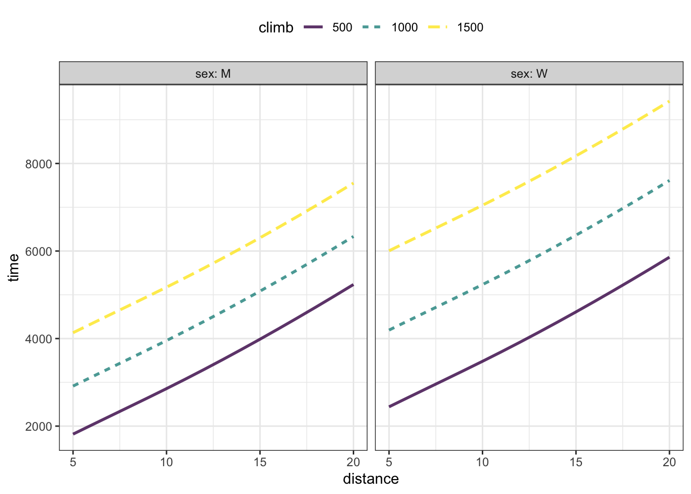
The friends decide on a baseline race: the hypothetical race to which they will add the 1 km or the 50 m. They decide that a race with a distance of 20 km and a climb of 1000 m sounds about right.
These baseline values are given as inputs to the model. As for the sex input to the model, they will do the calculation for females and males separately. Table ?? are the baseline results, where the model output is in seconds.
Baseline: Distance 20 km, climb 1000 m
##   distance climb sex model_output
## 1       20  1000   W         7612
## 2       20  1000   M         6333
Experiment 1: Add 1 km to the distance.
##   distance climb sex model_output
## 1       21  1000   W         7875
## 2       21  1000   M         6596
For females, the extra distance costs an extra 7875 - 7612 = 263 seconds. For males, the cost turns out to be the same: 6596 - 6333 = 263 seconds.
Experiment 2: Add 50 m to the climb.
##   distance climb sex model_output
## 1       20  1050   W         7792
## 2       20  1050   M         6450
For females, the extra climb costs 7792 - 7612 = 180 seconds. For males, the extra climb costs 6450 - 6333 = 117 seconds.
Overall, it seems that the extra kilometer is much harder than the extra climb, particularly for guys.11 NOTE IN DRAFT: Come back to this example when discussing interactions.
Amelia and Jack’s conversation turns to comparing their own race times. They often run together and finish the race at the same time. Is one of them a better runner than the other?
Amelia teases Jack that she is the better runner. After all, holding distance and climb at their baseline values, the model output differs between the sexes: 7612 seconds for women, 6333 for men.(See Table ??.) Amelia argues that if she were a man, her race time would be faster than Jack’s by about 7612 - 6333 = 1279 seconds.
An effect size quantifies the difference in model output when a single model input is changed. For categorical input va, variables like sex, the effect size is simply the difference in model outputs between two specified levels. So the effect size for winning time versus sex is 1279 seconds longer for women than men.
For quantitative input variables the effect size is formatted differently. Instead of a simple change in model output, the effect size is presented as a rate: the change in output divided by the change in input. For women, the effect size of winning time versus climb is
\[\frac{\mbox{change in output}}{\mbox{change in input}} = \frac{7792\ \mbox{s} - 7612\ \mbox{s}}{50\ \mbox{m}} = 3.6 \frac{\mbox{s}}{\mbox{m}} .\]
For men, the effect size of climb on winning time works out to be somewhat different. 6450 - 6333 = 117
\[\frac{\mbox{change in output}}{\mbox{change in input}} = \frac{6450\ \mbox{s} - 6333\ \mbox{s}}{50\ \mbox{m}} = 2.3 \frac{\mbox{s}}{\mbox{m}} .\]
The effect size of race distance on winning time is, for women,
\[\frac{\mbox{change in output}}{\mbox{change in input}} = \frac{7875\ \mbox{s} - 7612\ \mbox{s}}{1\ \mbox{km}} = 263 \frac{\mbox{s}}{\mbox{km}} .\]
An effect size always refers to the change in output when changing one explanatory variable and holding all the other variables constant. Calculating an effect size is analogous to doing an experiment on the model where the experiment involves changing just one variable.
An effect size describes a model. There can be different models of the same output. The explanatory variables might differ, for instance. The different models may well give different values for an effect size.
13.2 Interactions
Recall that the effect size of winning time with respect to climb was different for the two sexes. In other words, the effect size of one variable depends on the value of another variable. Such a link between the effect size of one explanatory variable and a second explanatory variable is called an interaction between the variables.[NOTE IN DRAFT: Technical point for computation notes: In some function families, such as the linear family of functions, it’s up to the modeler to declare whether the model should include an interaction. In other model families, interactions will be included naturally. For example, in the model time ~ distance + climb + sex examined in the previous section, I used the linear family of functions specifying that there should be an interaction between climb and sex but not between distance and sex. I made that choice only for pedagogical reasons: to show examples where there is and is not an interaction. We haven’t yet encountered the modeling tools to quide the decision about including interactions, but if your the question you seek to address with data is about an interaction (e.g., is the effect of climb different for men and women), you’ll need to be careful in using linear models to make sure that your model contains an interaction.]
Sometimes the question you want to answer is properly framed in terms of an interaction. For instance, is the effect of climb race outcome different for men and women? That’s a question about the existence of an interaction between climb and sex.12 NOTE IN DRAFT: Example: Interaction between Paxil (paroxetine) and prevastatin in raising glucose levels: Nicholas Tatonetti search of FDA adverse-reaction database.
13.3 Other formats for effect sizes
Different fields have different conventions for reporting effect sizes. As such, you may encounter the concept of effect size under different names. Some important ones:
In economics, an effect size is often presented as an elasticity. In an elasticity, the ratio is calculated using percentage change rather than absolute change.
For example, in the previous orange juice example, the price of oranges increased by 85 USD per ton from 850 USD per ton, an increase of 10%. Similarly, the demand changed from 50 to 46 million liters per year: a decrease of 8%. Consequently, the elasticity of demand for orange juice with price of oranges, is -8% / 10% or -0.80.
Elasticities do not have units because both the numerator and denominator are calculated as percent changes.
In public health and medicine, effect sizes for a categorical response variable are often presented as odds ratios. “Odds” are another way of describing probability. A probability \(p\) is the same as an odds \(p / (1 - p)\). So an effect size involving a change in probability \(p_2 - p_1\) would instead be presented as a ratio of odds: \[\mbox{odds ratio: } \frac{p_2 / (1 - p_2)}{p_1 / (1 - p_1)} .\] An odds ratio of 1 means “no change.”
13.4 Intervals for effect sizes
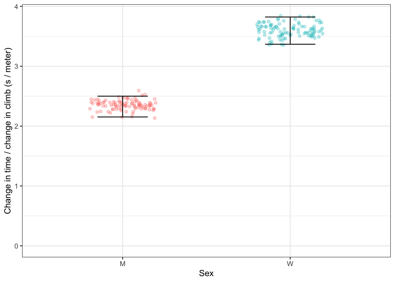
Figure 13.2: The effect size for climb on winning time for the two sexes. Effect sizes ought to be presented as an interval. The techniques to construct such intervals are introduced in Chapters ?? and 20.
In the preceeding sections, I’ve presented effect sizes as a single quantity. It’s better to present them as an interval, just as predictions can be given as an interval. We’ll encounter the techniques for finding the interval in Chapters ?? and 20. Figure 13.2 shows a 95% interval, called a confidence interval on the effect size of climb on winning time.
13.5 Effect sizes and interventions
An effect size is a way of describing a model. There need be no presumption that the model itself respects the actual causal mechanisms at work in the system. For instance, in a classifier built to screen for cancer, the model inputs might be physical signs of cancer such as the presence of a chemical antigen or high-density tissue found in an X-ray. The model inputs are therefore the consequence of the cancer, not the cause. But even though such a model gets causation exactly backwards, the model may be useful in providing a way to detect a condition that is not directly observable.
In many situations, the model has been built with specific intention to capture the genuine causal connections in the system. (Chapter 6 introduces some techniques for accomplishing this.) When this is the case, an effect size provides a way to anticipate the effect of an intervention. For instance, a company is deciding whether to raise the price of its product. That price change will presumably cause demand for the product to go down which, in turn, will affect the revenue generated by the product. An effect size of (input) price on the (output) revenue indicates what the result of the price-changing intervention will be on revenue.
Sometimes the causal relationship between an explanatory variable and the response variable is self-evident. Increased wind velocity of hurricanes leads to more damage. Sometimes there is a complex web of causality of the sort seen in Chapter @ref(causal_networks). Often, there is controversy about what causes what, for instance does increased parental involvement lead to better teaching materials or is this just a matter of funding. Merely building a predictive model is no guarantee that an effect size will be predictive of the outcome when we actually change an input to the system. In later chapters, we’ll introduce ways to determine whether an effect size does indeed correspond to the real-world causal mechanisms at work.
13.6 Exercises
Problem 1: Over the past hundred years, attitudes toward sex have changed. Let’s examine one way that this change might show up in data: the age at which people first had sex. The National Health and Nutrition Evaluation Survey includes a question about the age at which a person first had sex. For the moment, let’s focus just on that subset of people who have had sex at least once.
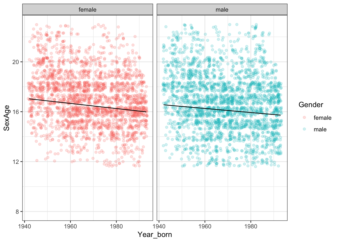
What is the effect size of year born on age at first sex? Use units of years-over-years.
Is there evidence for an interaction between gender and year born?
Translate the effect size in (1) to the units weeks-over-years.
Problem 2: The logic of effect size is to investigate the change in output of a model when one input variable is changed, holding all other things constant. This problem is about the extent to which we mean “all”.
The figure shows yearly CO2 production of individual gasoline-fueled passenger vehicles stratified by the number of engine 4 or 6 cylinders.
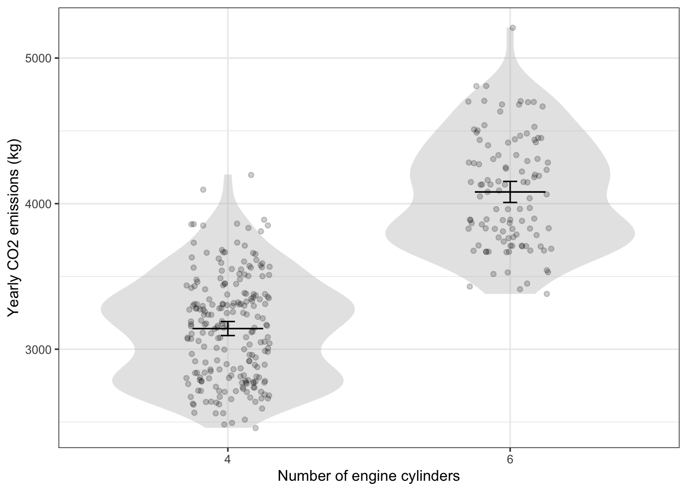
- The effect size is the difference between the output variable when a change is made to an input. Consider the effect size of changing from a six-cylinder engine to a four-cylinder engine. Here’s a subtly incorrect way of calculating something like an effect size: Pick a dot from the six-cylinder group and another dot from the four-cylinder group. Subtract the 4-cylinder point’s CO2 value from the six-cylinder point’s CO2 value, and divide by the change in the input, that is, -2 cylinders.
- Follow this procedure for the top-most dot in each cloud and calculate the effect size.
- Follow the procedure for the bottom-most dot in each cloud and calculate the effect size.
- Follow the procedure for the bottom-most dot in the four-cylinder cloud and the top-most dot in the six-cylinder cloud.
- Do the same as in (c) but use the bottom-most six-cylinder dot and the top-most four-cylinder dot.
- You can imagine the (tedious) process of repeating the calculation for every possible pair of dots and getting a distribution of effect sizes. What would be the range of this distribution: from the smallest effect size to the biggest? (Hint: You can figure it out from your answers to (1).)
From your result in (2), you might be tempted to conclude that the effect size is highly uncertain: it might be negative or it might be positive. But there is a problem, the procedure used in (1) and (2) fails to incorporate the notion of all other things being equal. This notion applies not just to known variables, but to all the other unknown factors that shape the data.
For the purpose of envisioning the concept, imagine that we actually had a measurement of all the factors that shaped CO2 emissions from a vehicle. We’ll call this imaginary measurement “all other things”. The figure below shows a conceptualization of what CO2 emissions as a function of the number of cylinders and “all other things” would look like.
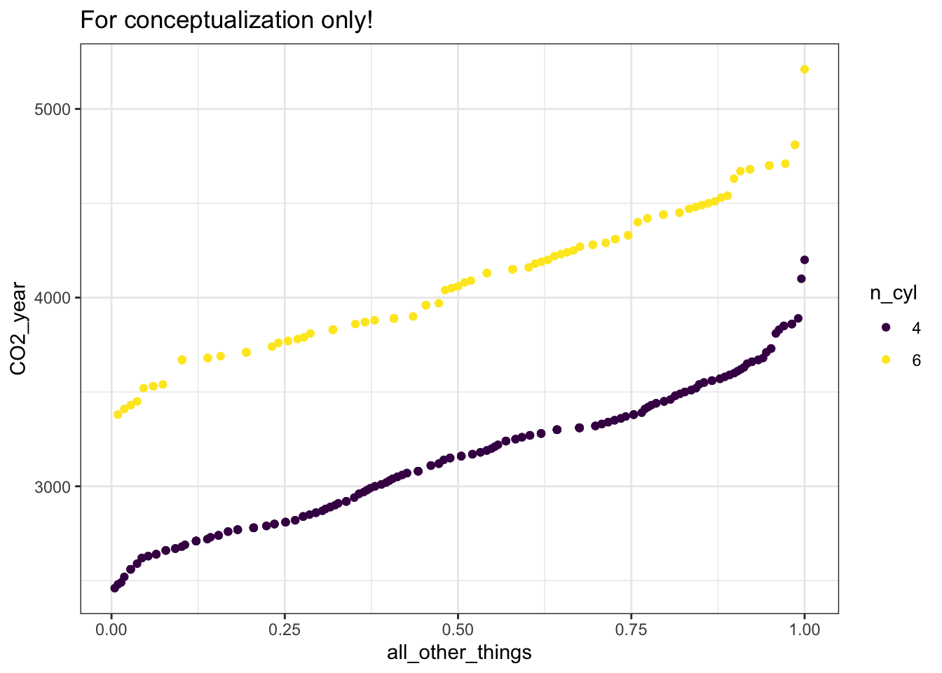
- Using the graph of CO2_year versus “all other things”, calculate the effect size of a change from six to four cylinders. Remember to hold “all other things” constant in your calculations. So do the effect size calculation at each of several values of “all other things”. What is the effect size and about how much does it vary from one value of “all other things” to another?
This exercise is intended to give you a way of thinking about effect size and “all other things”. In reality, of course, we do not have a way to measure “all other things”. Instead, we calculate the effect size not directly from the data but from the model output (indicated by the statistic layer in the first graphic). As we saw in Chapter @ref(sampling_variation), there is actually some uncertainty about the model output stemming from sampling variability that can be summarized by a “confidence interval”. For the relationship between the number of cylinders and CO2 emissions, the extent of that uncertainty is indicated by the interval layer in the first graphic. A fair depiction for the corresponding uncertainty in the effect size can be had by repeating the process of (2), but only for points falling into the confidence interval.
Problem 3: The National Cancer Institute publishes an online, interactive “Breast Cancer Risk Assessment Tool”, also called the “Gail model.” The output of the model is a probability that the woman whose characteristics are used as input will develop breast cancer in the next five years. The inputs include:
- age
- race/ethnicity
- age at first menstrual period
- age at birth of first child (if any)
- how many of the woman’s close relatives (mother, sisters, or children) have had breast cancer
As a baseline, consider a 55-year-old, African-American woman who has never had a breast biopsy or any history of breast cancer, who doesn’t know her BRCA status, and whose close relatives have no history of breast cancer, whose first menstrual period was at age 13 and first child at age 23. No “subrace” or “place of birth” is specified.
Follow the link above to the cancer risk assessment tool, and enter the baseline values into the assessment tool using the link above. According to the assessment tool, what is the probability (“risk”) of developing breast cancer in the next five years? What is the lifetime risk of developing breast cancer?
What is the effect size on our baseline subject of finding out that:
- one of her close relatives has developed breast cancer?
- more than one of her close relatives have developed breast cancer?
What is the effect size associated with comparing the baseline conditions to a woman with the same conditions but a race of white?
What is the effect size of age? Compare the baseline 55-year old woman to herself when she is 65, without the other inputs changing. Since age is quantitative, Report the effect size as percentage-points-per-year.
Problem 4: Start content here.
Referring to Figure 10.9 identify any situations where the effect size of wind direction is large. That is, holding the other variables (barometric pressure, temperature, wind speed), find two different wind-directions that have very different values for the probability output of the model.
Elasticity of college GPA with standardized test score. Using r = 0.4, a 10% higher test score would be associated with a 4% higher GPA.