Chapter 16 Model performance
We encounter predictions in everyday life and work: what will be the high temperature tomorrow, what will be the sales of a product, what will be the price of fuel, how large will be the harvest of grain at the end of the season, and so on. Often such predictions come from authoritative sources: the weather bureau, the government, think tanks. These predictions, like those that come from our own statistical models, are likely to be somewhat off target from the actual outcome.
This chapter introduces a simple, standard way to quantify the size of prediction errors: the root mean square prediction error (RMSE). Those five words are perhaps a mouthful, but as you’ll see, “root mean square” is not such a difficult operation.
16.1 Prediction error
We often think of “error” as the result of a mistake or blunder. That’s not really the case for prediction error. Prediction models are built using the resources available to us: explanatory variables that can be measured, accessible data about previous events, our limited understanding of the mechanisms at work, and so on. Naturally, given such flaws our predictions will be imperfect. It seems harsh to call these imperfections an “error”. Nonetheless, Prediction error is the name given to the deviation between the output of our models and the way things eventually turned out in the real world.
The use we can make of a prediction depends on how large those errors are likely to be. We have to say “likely to be” because, at the time we make the prediction, we don’t know what the actual result will be. Chapter 5 introduced the idea of a prediction interval: a range of values that we believe the actual result is highly likely to be in. “Highly likely” is conventionally taken to be 95%.
It may seem mysterious how one can anticipate what an error is likely to be, but the strategy is simple. In order to guide our predictions of the future, we look at our records of the past. The data we use to train a statistical model contains the values of the response variable as well as the explanatory variables. This provides the opportunity to assess the performance of the model. First, generate prediction outputs using as inputs the values of the explanatory variables, Then, compare the prediction outputs to the actual value of the response variable.
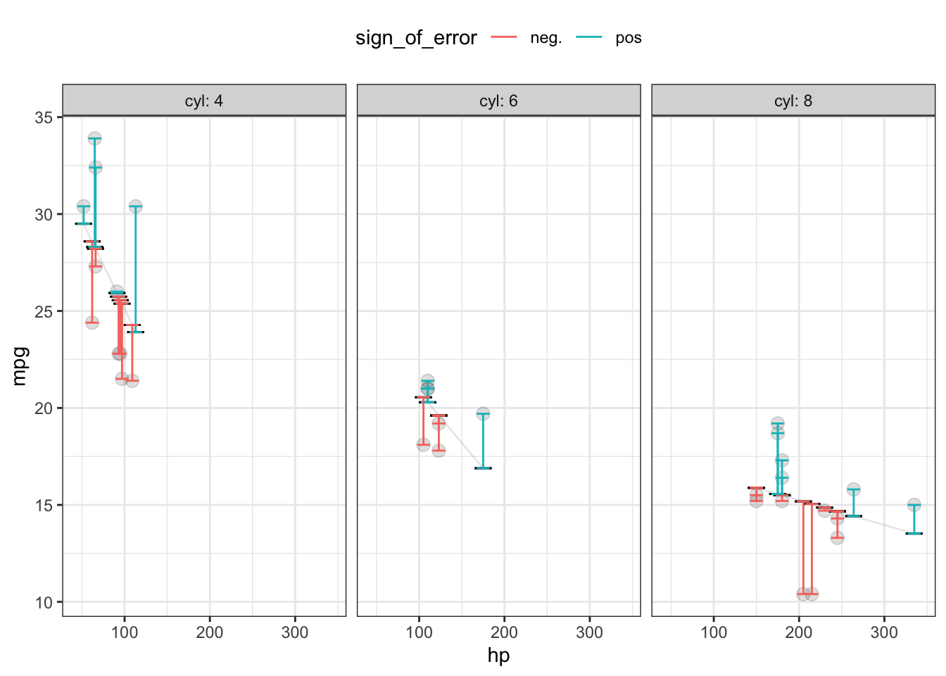
The comparison process is illustrated in Table 16.1 and, equivalently, Figure 16.1. The error is the numerical difference between the actual response value and the model output. The error is calculated from our data on a row-by-row basis: one error for each row in our data. The error will be positive when the actual response is larger than the model output, negative when the actual response is smaller, and would be zero if the actual response equals the model output.
Table 16.1: Prediction error from a model mpg ~ hp + cyl of automobile fuel economy versus engine horsepower and number of cylinders. The actual response variable, mpg, is compared to the model output to produce the error and square error.
| hp | cyl | mpg | model_output | error | square_error |
|---|---|---|---|---|---|
| 110 | 6 | 21.0 | 20.29 | 0.71 | 0.51 |
| 110 | 6 | 21.0 | 20.29 | 0.71 | 0.51 |
| 93 | 4 | 22.8 | 25.74 | -2.94 | 8.67 |
| 110 | 6 | 21.4 | 20.29 | 1.11 | 1.24 |
| 175 | 8 | 18.7 | 15.56 | 3.14 | 9.85 |
| 105 | 6 | 18.1 | 20.55 | -2.45 | 6.00 |
| … and so on for 32 rows altogether. |
Figure 16.1: A graphical presentation of Table 16.1. The data layer presents the actual values of the input and output variables. The model output is displayed in a statistics layer by a dash. The error is shown in an interval layer. To emphasize that the error can be positive or negative, color is used to show the sign.
Once each row-by-row error has been found, we consolidate these errors into a single number representing an overall measure of the performance of the model. One easy way to do this is based on the square error, also shown in Table 16.1 and Figure 16.1. The squaring process turns any negative errors into positive square errors.
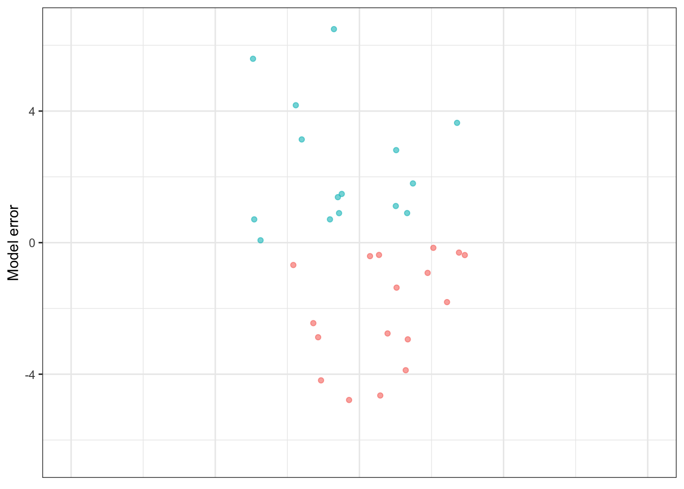
Figure 16.2: The prediction errors and square errors corresponding to Table 16.1 and Figure 16.1. The color shows the sign of the error. Since errors are both positive and negative in sign, overall they are centered on zero. But square errors are always positive, so the mean square error is positive.
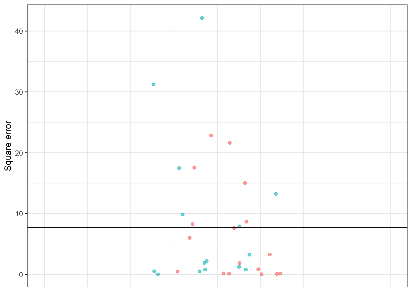
Adding up those square errors gives the so-called sum of square errors (SSE). The SSE depends, of course, on both how large the individual errors are and how many rows there are in the data. For Table 16.1, the SSE is 247.61 miles-per-gallon.
The mean square error (MSE) is the average size of the square errors, for example dividing the sum of square errors by the number of rows in the data frame. In Table 16.1, the MSE is simply the SSE divided by the number of rows in the data frame. In Table 16.1 the MSE is 247.61 / 32 = 7.74 square-miles per square-gallon.
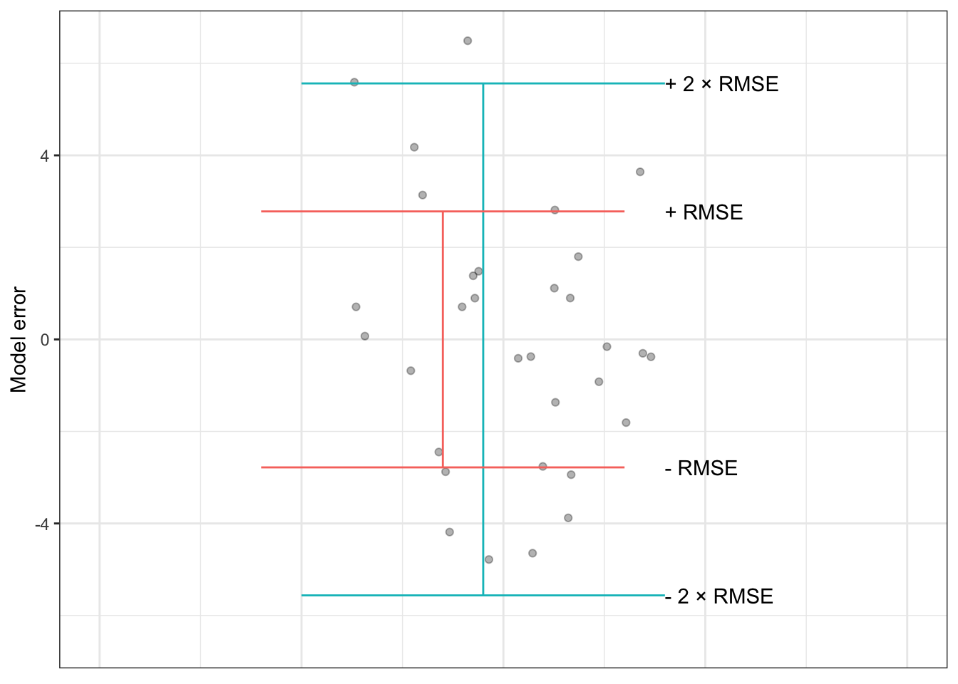
Figure 16.3: The model errors from Table 16.1 shown along with interval ± RMSE and ± 2 × RMSE. The shorter interval encompasses about 67% of the errors, the longer interval covers about 95% of the errors.
Yes, you read that right: square-miles per square-gallon. It’s important to keep track of the physical units of a prediction. These will always be the same as the physical units of the response variable. For instance, in Table 16.1, the response variable is in terms of miles-per-gallon, and so the prediction itself is in miles-per-gallon. Similarly, the prediction error, being the difference between the response value and the predicted value, is in the same units, miles-per-gallon.
Things are a little different for the square error. Squaring a quantity changes the units. For instance, squaring a quantity of 2 meters gives 4 square-meters. This is easy to understand with meters and square-meters; squaring a length produces an area. (This length-to-area conversion is the motivation behind using the word “square.”) For other quantities, such as time, the units are unfamiliar. Square the quantity “15 seconds” and you’ll get 225 square-seconds. Square the quantity “11 chickens” and you’ll get 121 square-chickens. This is not a matter of being silly, but of careful presentation of error.
A mean square error is intended to be a typical size for a square error. But the units, for instance square-miles-per-square-gallon in Table 16.1, can be hard to visualize. For this reason, most people prefer to take the square root of the mean square prediction error. This changes the units back to those of the response variable, e.g. miles-per-gallon, and is yet another way of presenting the magnitude of prediction error.
The root mean square error (RMSE) is simply the square root of the mean square prediction error. For example, in Table 16.1, the RMSE is 2.78 miles-per-gallon, which is just the square root of the MSE of 7.74 square-miles per square-gallon.
16.2 Prediction intervals and RMSE
As described in Chapter 5, predictions can be presented as a prediction interval sufficiently long to cover the large majority of the actual outputs. Another way to think about the length of the prediction interval is in terms of the magnitude typical prediction error. In order to contain the majority of actual outputs, the prediction interval ought to reach upwards beyond the typical prediction error and, similarly, reach downwards by the same amount.
The RMSE provides an operational definition of the magnitude of a typical error. So a simple way to construct a prediction interval is to fix the upper end at the prediction function output plus the RMSE and the lower end at the prediction function output minus the RMSE.
It turns out that constructing a prediction interval using ± RMSE provides a roughly 67% interval: about 67% of individual error magnitudes are within ± RMSE of the model output. In order to produce an interval covering roughly 95% of the error magnitudes, the prediction interval is usually calculated using the model output ± 2 × RMSE.
This simple way of constructing prediction intervals is not the whole story. Another component to a prediction interval is “sampling variation” in the model output. Sampling variation will be introduced in Chapter 15.
16.3 Training and testing data
When you build a prediction model, you have a data frame containing both the response variable and the explanatory variables. This data frame is sometimes called the training data, because the computer uses it to select a particular member from the modeler’s choice of the family of functions for the model, that is, to “train the model.”
In training the model, the computer picks a member of the family of functions that makes the model output as close as possible to the response values in the training data. As described in Chapter 15, if you had used a new and different data frame for training, the selected function would have been somewhat different because it would be tailored to that new data frame.
In making a prediction, you are generally interested in events that you haven’t yet seen. Naturally enough, an event you haven’t yet seen cannot be part of the training data. So the prediction error that we care about is not the prediction error calculated from the training data, but that calculated from new data. Such new data is often called testing data.
Ideally, to get a useful estimate of the size of prediction errors, you should use a testing data set rather than the training data. Of course, it can be very convenient to use the training data for testing. Sometimes no other data is available. Many statistical methods were first developed in an era when data was difficult and expensive to collect and so it was natural to use the training data for testing. A problem with doing this is that the estimated model error will tend to be smaller on the training data than on new data. To compensate for this, as described in Chapter 21, statistical methods used careful accounting, including quantities such as “degrees of freedom,” to compensate mathematically for the underestimation in the error estimate.
Nowadays, when data are plentiful, it’s feasible to split the available data into two parts: a set of rows used for training the model and another set of rows for testing the model. Even better, a method called cross validation effectively lets you use all your data for training and all your data for testing, without underestimating the prediction model’s error. Cross validation is discussed in Chapter 18.
16.4 Example: Predicting winning times in hill races
The Scottish hill race data contains four related variables: the race length, the race climb, the sex class, and the winning time in that class. Figures 10.7 and 10.8 in Section ?? show two models of the winning time:
Suppose there is a brand-new race trail introduced, with length 20 km, climb 1000 m, and that you want to predict the women’s winning time.
Using these inputs, the prediction function output is
time ~ lengthproduces output 7400 secondstime ~ length + climb + sexproduces output 7250 seconds
It’s to be expected that the two models will produce different predictions; they take different input variables.
Which of the two models is better? One indication is the size of the typical prediction error for each model. To calculate this, we use some of the data as “testing data” as in Tables 16.2 and 16.3. With the testing data (as with the training data) we already know the actual winning time of the race, so calculating the row-by-row errors and square errors for each model is easy.
Table 16.2: time ~ distance: Testing data and the model output and errors from the time ~ distance model. The mean square error is 1,861,269, giving a root mean square error of 1364 seconds.
| distance | climb | sex | time | model_output | error | square_error |
|---|---|---|---|---|---|---|
| 20.0 | 1180 | M | 7616 | 7410 | 206 | 42,436 |
| 20.0 | 1180 | W | 9290 | 7410 | 1880 | 3,534,400 |
| 19.3 | 700 | M | 4974 | 7143 | -2169 | 4,704,561 |
| 19.3 | 700 | W | 5749 | 7143 | -1394 | 1,943,236 |
| 21.0 | 520 | M | 5299 | 7791 | -2492 | 6,210,064 |
| 21.0 | 520 | W | 6101 | 7791 | -1690 | 2,856,100 |
| … and so on for 46 rows altogether. |
Table 16.3: time ~ distance + climb + sex: Testing data and the model output and errors from the time ~ distance + climb + sex model. The mean square error is 483,073 square seconds, giving a root mean square error of 695 seconds.
| distance | climb | sex | time | model_output | error | square_error |
|---|---|---|---|---|---|---|
| 20.0 | 1180 | M | 7616 | 6422 | 1194 | 1,425,636 |
| 20.0 | 1180 | W | 9290 | 7856 | 1434 | 2,056,356 |
| 19.3 | 700 | M | 4974 | 5360 | -386 | 148,996 |
| 19.3 | 700 | W | 5749 | 6525 | -776 | 602,176 |
| 21.0 | 520 | M | 5299 | 5341 | -42 | 1,764 |
| 21.0 | 520 | W | 6101 | 6488 | -387 | 149,769 |
| … and so on for 46 rows altogether. |
Using the testing data, we find that the root mean square error is
time ~ lengthhas RMSE 1364 secondstime ~ length + climb + sexhas RMSE 695 seconds
Clearly, the time ~ length + climb + sex model produces better predictions than the simpler time ~ length model.
The race is run. The women’s winning time turns out to be 8034 sec. Were the predictions right?
Obviously both predictions, 7250 and 7400 secs, were off. You would hardly expect such simple models to capture all the relevant aspects of the race (the weather? the trail surface? whether the climb is gradual throughout or particularly steep in one place? the abilities of other competitors). So it’s not a question of the prediction being right on target but of how far off the predictions were. This is easy to calculate: the length-only prediction (7400 sec) was low by 634 sec; the length-climb-sex prediction was low by 784 sec.
If the time ~ distance + climb + sex model has an RMSE that is much smaller than the RMSE for the time ~ distance model, why is it that time ~ distance had a somewhat better error in the actual race? Just because the typical error is smaller doesn’t mean that, in every instance, the actual error will be smaller.
16.5 Example: Exponentially cooling water
Back in Figure ??, we displayed data on temperature versus time data of a cup of cooling water. To model the relationship between temperature and time, we used a flexible function from the linear family. A physicist might point out that cooling often follows an exponential pattern and that a better family of functions would be the exponentials. Although exponentials are not commonly used in statistical modeling, it’s perfectly feasible to fit a function from that family to the data. The results are shown in Figure 16.4 for two different exponential functions, the flexible linear function of Figure ??, and a super-flexible linear function.
Figure 16.4: The temperature of initially boiling water as it cools over time in a cup. The thin lines show various functions fitted to the data: a stiff linear model, a flexible linear model, a special-purpose model of exponential decay.
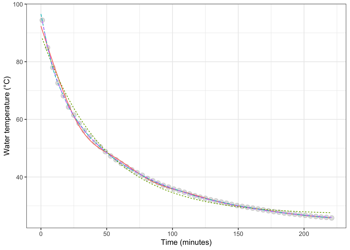
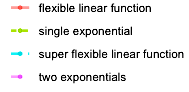
Figure 16.5: The model error – that is, the difference between the measured data and the model values – for each of the cooling water models shown in Figure 16.4.
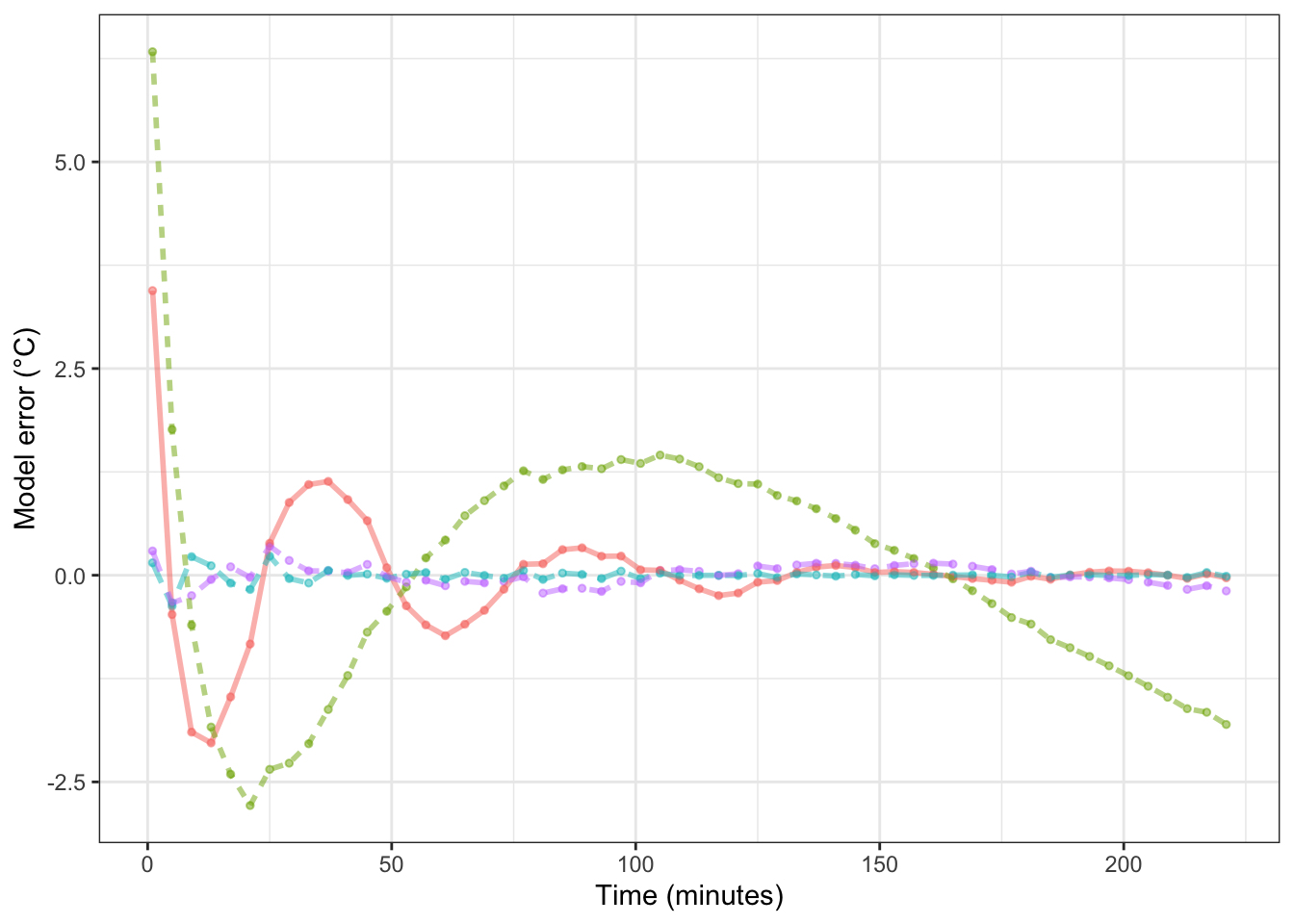
Table 16.4: The root mean square error (RMSE) for four different models of the temperature of water as it cools. The training data, not independent testing data, was used for the RMSE calculation
| model | RMSE |
|---|---|
| super flexible linear function | 0.0800 |
| two exponentials | 0.1309 |
| flexible linear function | 0.7259 |
| single exponential | 1.5003 |
To judge from solely from the RMSE, the super flexible linear function model is the best. In Chapter 18 we’ll examine the extent to which that result is due to using the training data for calculating the RMSE.
Keep in mind, though, that whether a model is good depends on the purpose for which it is being made. For a physicist, the purpose of building such a model would be to examine the physical mechanisms through which water cools. A one-exponential model corresponds to the water cooling because it is in contact with one other medium, such as the cup holding the water. A two-exponential model allows for the water to be in contact with two, different media: a fast process involving the cup and a slow process involving the room air, for instance. The RMSE for the two-exponential model is much smaller than for the one-exponential model, providing evidence that there are at least two, separate cooling mechanisms at work.