Chapter 11 Models that learn
Chapters 4 and 10 introduced three different families of functions for constructing predictive models.
- Unbounded functions. There are many techniques. In this book we are using arithmetic combinations of the explanatory variables, which can be either quantitative or categorical. The output is a number, so unbounded functions are well suited when the response variable is quantitative.
- Bounded functions. These work much like unbounded functions, but the output is post-processed to be between zero and one. As such, bounded functions are a good choice when the response variable is categorical. (Remember, for categorical response variables, the model output will be a probability assigned to each possible level of the variable.)
- Stratification by all the combinations of the explanatory variables. This works when all the explanatory variables are categorical. (You can change a quantitative variable into quantitative by chopping up the number line into discrete segments.) The output of a stratification model can be whatever you like. Thus, stratification models can handle response variables that are either quantitative or categorical.
This chapter introduces yet another family of models: tree models.10 Also called classification and regression trees or recursive partitioning.
Like linear or logistic models, tree models can make direct use of both quantitative and categorical explanatory variables. Like stratification, the output can be whatever you like, so tree models are suitable for both quantitative and categorical response variables.
Tree models are part of a large collection of model families called machine learning models. The “machine”, of course, is the computer. What’s new in these model families is “learning”.
Machine learning models characteristically involve exploration of possibilities and decision making about what new directions to explore given the results of earlier explorations. As you’ll see, the “exploring” done in building tree models is simple and systematic. Similarly the “decision making” amounts to selecting a single one of the explored possibilities and continuing to explore from there.
11.1 Trees and stratification
Table 11.1: Data on age, smoking, and mortality over a 20-year follow-up. (Available as a data frame in mosaicData::Whickham.) age_group is a categorical version of age which will be used in the stratification seen in Table 11.2.
| age | age_group | smoker | outcome |
|---|---|---|---|
| 56 | 40 to 60 | No | Dead |
| 54 | 40 to 60 | Yes | Alive |
| 21 | under 40 | Yes | Alive |
| 72 | over 60 | No | Dead |
| 30 | under 40 | Yes | Alive |
| 19 | under 40 | No | Alive |
| … and so on for 1,314 rows altogether. |
To start, let’s compare tree models to the other function families so that you can see what the “exploration” in machine learning turns up. To do this, we will build models of mortality as a function of age and smoking. The data (Table 11.1) come from a study in which people were interviewed and, among other things, each person’s age and whether or not they smoke was recorded. Twenty years after the interview, a follow-up study checked whether the person was still alive. This outcome is a categorical variable with two levels: alive or dead. We use three different function families to model outcome ~ age + smoking: a stratification, a logistic model, and a tree model.
Table 11.2: A stratification of Table 11.1 using explanatory variables age_group and smoker.
| smoker | age_group | prop_alive | n_rows |
|---|---|---|---|
| No | under 40 | 96.9 | 289 |
| Yes | under 40 | 96.6 | 236 |
| No | 40 to 60 | 79.6 | 201 |
| Yes | 40 to 60 | 72.7 | 245 |
| No | over 60 | 25.6 | 242 |
| Yes | over 60 | 36.6 | 101 |
In constructing the stratification, we need to convert the quantitative variable age into a categorical variable. There are many ways in which this can be done: five year intervals, age decades, “young” vs “old” and so on. We’ll use three levels based on common sense definitions of “stages” of life: under 40, between 40 and 60, over 60. The categorical variable, age_group with these three levels is included in Table 11.1. The stratification itself is a simple matter of tabulating what fraction of people are alive in each of the six combinations of age_group and smoker, as shown in Table 11.2.
The stratification model shown in Table 11.2 can also be displayed graphically, as in Figure 11.1.
Figure 11.1: The stratification model presented graphically.
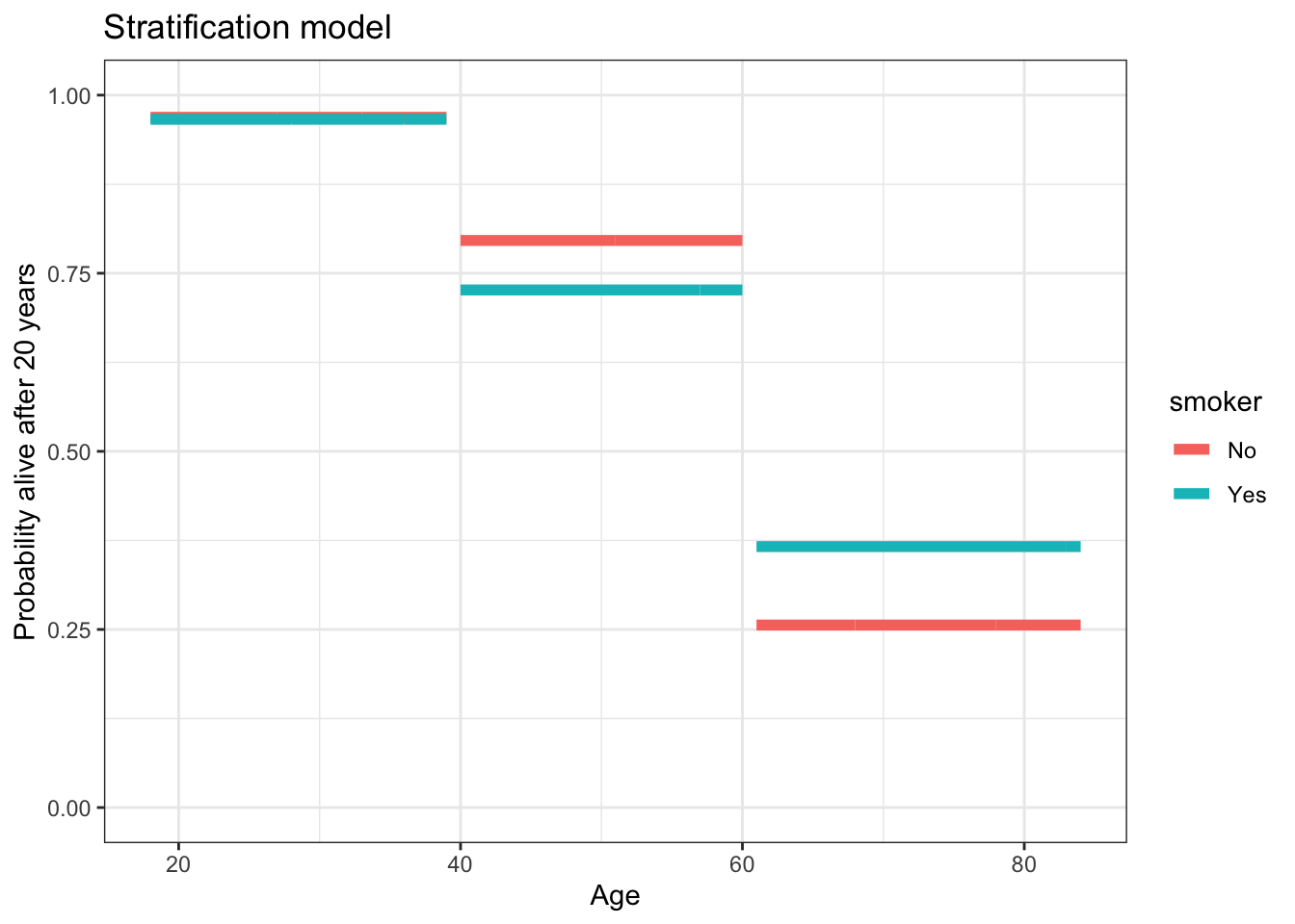
The model graphed in 11.1 is based on our choice of the age groups “under 40”, “40-60”, “over 60”. Had we selected a different number of groups or different division points between groups, the model would be different. The stratification method doesn’t explore other possibilities, although the modeler is certainly free to build many stratification models and compare them.
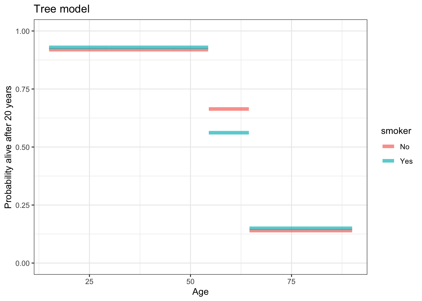
The point of machine learning models is to explore the various possibilities. A tree model outcome ~ age + smoker does this. The results of the exploration are shown graphically in Figure 11.2 and, equivalently, in Table 11.3. The model has learned how to define the strata, rather than the strata being set by pre-defined groups.
Figure 11.2: The graph of the tree model outcome ~ smoker + age. For those younger than 55 and those older than 64, the probability of being alive is the same for smokers and non-smokers.

Table 11.3: A tree model of outcome ~ age + smoker.
| age | smoker | Prob. alive | n rows | n alive |
|---|---|---|---|---|
| 54 or younger | 92% | 833 | 766 | |
| 55 to 64 | No | 66% | 122 | 81 |
| 55 to 64 | Yes | 55% | 116 | 25 |
| 65 or older | 14% | 243 | 34 |
It’s important to note that the tree model is a kind of stratification. But rather than breaking up the data into all the different strata implied by smoker and age_decade, the tree model is exploring different ways of defining the strata and picking one it regards as best. The number of rows in the strata vary from 833 to 122. For the oldest and youngest people in Whickham, smoking status is not used in the partitioning; according to the model, smoking only shows up as affecting survival for those aged 55 to 64.
Finally, consider a logistic model of outcome ~ smoker + age. Recall that a logistic model is a continuous function of any quantitative variable. The logistic function is graphed in Figure ??.
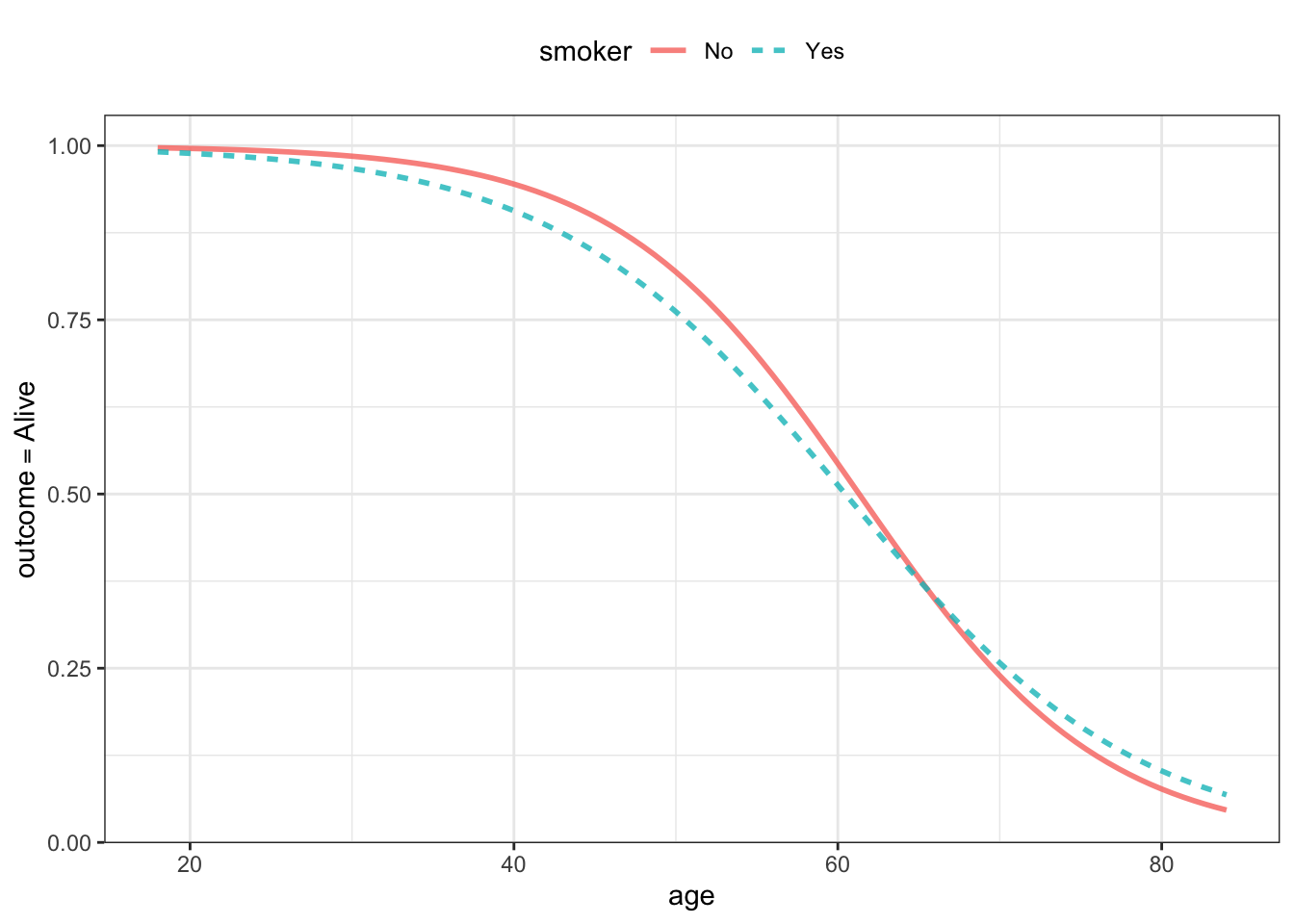
The differences between the three models – stratification, tree, logistic – based on exactly the same data raise an extremely important statistical question: Which “details” of the functions are we to take seriously and which not? For example, in the stratification model, smokers over 60 are seen to have a higher probability of survival than non-smokers. This pattern is also seen to a smaller extent in the logistic function. The tree model, on the other hand, does not show this higher probability survival for smokers over 60.
The statistical approach to deciding what details of a model function to take seriously is introduced starting in Chapter 15.
11.2 Growing trees
Neither Figure 11.2 nor Table 11.3 looks very much like a tree. Describing such models with the metaphor of a tree reflects how the models are constructed, as a series of divisions of rows into two groups. The rows are the equivalent of leaves. Each leaf is carried on a branch, the branch itself stems from a bigger branch, and so on down to the trunk, which carries all the leaves.
The process of constructing a tree model starts with all the data rows. These are split into two groups, much as a trunk splits into two branches. Each of the two groups is considered separately and itself divided into two branches. As seen in Figure 11.3, the first step in the series of splits that led to the stratification in Table 11.3 was to split the data rows into two groups by age: those 65 and older versus everyone else. The computer determined that there is no added value in dividing up the 65-and-older into sub-groups, but it did find it meaningful to split the younger group into those 54 and younger and those 55 and older. Only for that last group, those 55 to 64, did the computer find a difference between smokers and non-smokers worth reporting.
Figure 11.3: The stratification in the Whickham tree model of Table 11.3, dividing the data rows into six distinct groups.
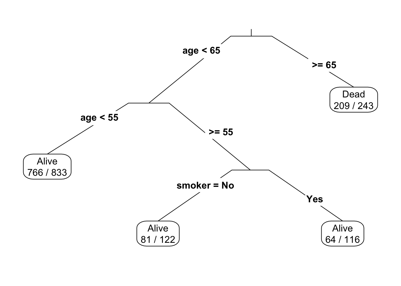
Although real trees grow from the ground up, in graphing trees we follow the convention of reading from the top of the page downward. So in Figure 11.3 the trunk is drawn at the top.
It takes some practice to learn to read tree diagrams. One way to approach the task is to think of a specific case, say a 63-year old smoker. This person goes to the left on the first split, since 63 is less than 65. On the next split, the person goes to the right, since 63 is greater than 55. The next split is between smokers and non-smokers. Our 63-year old goes to the right since she’s a smoker.
Another example: a 72-year old smoker. At the top, this person goes to the right branch, since 72 is greater than 65. That’s the end of the story, since the 65-and-older group is not split further. Notice that our 72-year old’s smoking status didn’t enter into the result, which is a probability of having died of 209/243 = 84%.
Table 11.4: The model resulting from stratifying by smoker. This model will be compared to all the other ways of subdividing the data using a single explanatory variable.
| smoker | prop_alive | n_rows |
|---|---|---|
| No | 68.6 | 732 |
| Yes | 76.1 | 582 |
How did the computer determine that the first split will be at age 65? When starting out, the computer could define the split either by smoker or by age. Trying out the split by smoker produced the stratification of Table 11.4. As for splitting by age, the computer needed to specify a particular age at which to make the split. Remarkably, the tree-building algorithms tests out all the possibilities: split at age 18, split at age 19, split at age 20, and so on. Two of these many possibilities are shown in Tables 11.5 and 11.6.
Table 11.5: Stratifying by whether the person is 42 or older.
| age | prop_alive | n_rows |
|---|---|---|
| 42 or older | 54 | 754 |
| less than 42 | 97 | 560 |
Table 11.6: Stratifying by whether the person is 65 or older.
| age | prop_alive | n_rows |
|---|---|---|
| 65 or older | 54 | 754 |
| less than 65 | 97 | 560 |
The tree-growing algorithm now calculates how well each of these candidate prediction models perform, that is, how well the model predictions match the actual outcomes. For now, however, you can think about the evaluation of the models in terms of the difference in model output for the two strata for each model. For the split at age 65, the difference is 84% - 14% = 70 percentage points. For the split at age 42, that difference is 97% - 54% = 43 percentage points. For the split by smoker, the difference is 76% - 69% = 7 percentage points. The split at age 65 wins!
Having made that split at age 65, the computer applies the same process, separately, to the data for the under 65s and the data for the 65+. Each time the computer has some data to split, it tries all the possibilities offered by the explanatory variables. It chooses the one that produces the best predictive model for the data it is splitting.
This splitting process can continue until there is a separate strata for every possible combination of age and smoker.
When looking at each stratum, the computer has another option available: Don’t split up the data. You can see this in Figure 11.3, where the computer declined to make any further splits among the 65+ group. As you might anticipate, the computer makes such a choice when it determines that further splitting is not statistically worthwhile, that is, that the predictive model produced by further splitting can be expected to perform no better (or even worse) than the predictive model with no further splitting.
11.3 Exercises
Problem 1: Here is a stratification table of the probability of surviving 20 year versus age and smoking status (using the mosaicData::Whickham data frame).
age |
smoker |
Prob. alive | n rows | n alive |
|---|---|---|---|---|
| \(\leq 45\) | 92% | 833 | 766 | |
| 45 to 64 | No | 66% | 122 | 81 |
| 45 to 64 | Yes | 35% | 116 | 25 |
| \(\geq 65\) | 14% | 243 | 34 |
And here is a graphic.
The graphic and the stratification table are inconsistent with one another. Fix the stratification table so that it matches the graphic.
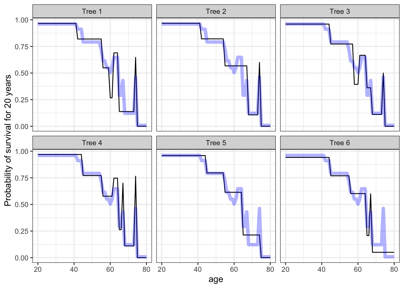
Problem 2 Tree models are very easy to construct and avoid any need to make explicit decisions about the flexibility of the model or interactions between explanatory variables. For instance, in Figure 11.1, the diminished survival of smokers among the people in their late 50s emerges without any need to specify that the model include an interaction between age and smoking status. On the other hand, the sharp transitions in the model output seem unnatural and potentially misleading.
The cleverly named random forest architecture attempts to mitigate the shortcomings of the tree architecture while retaining the advantages. A real forest is a collection of trees. A random forest model is a collection of tree models, typically 500 or so. In order to create variation among the individual tree models, each individual model is constructed from a a random resample of the data and, similarly, the subset of explanatory variables used in the individual models is selected with some degree of randomness. The figure below shows six individual tree models that went into the random forest. The random-forest model is also shown in each panel.
- Which of the lines in the panels is the individual tree model and which is the random-forest model. How can you tell?
Figure 11.4: Six trees from a random forest.
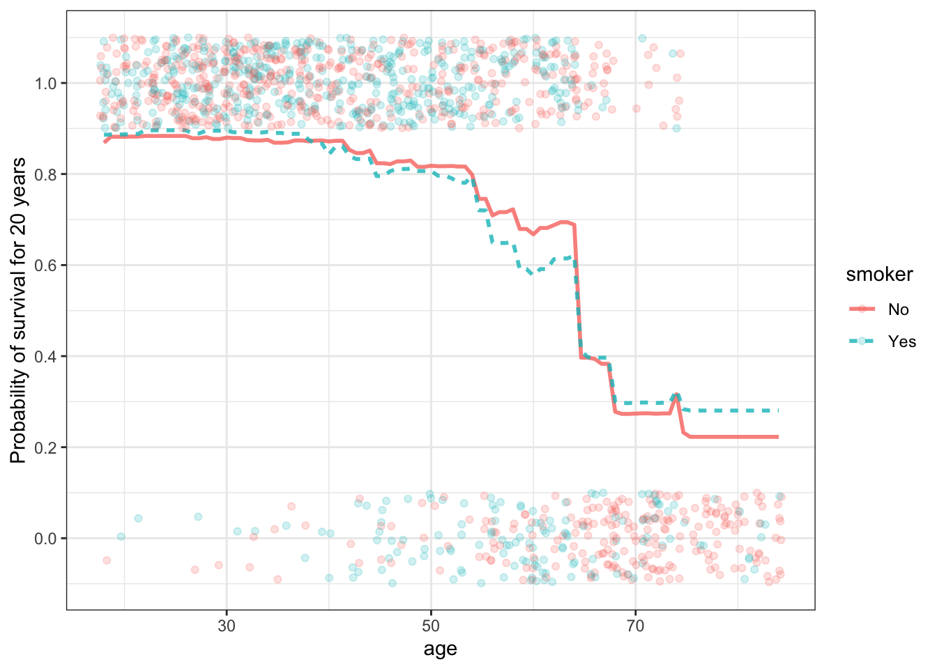
The figure below shows a random forest model of survival as a function of age and smoking status. The model function is somewhat jagged, reflecting the sharp transitions between plateaus in each of the individuals trees in the forest. Those transitions are diminished because the outputs of all the individual trees are averaged to give the output for the random forest. This results in many small transitions. since each individual tree can have its transitions in a different location than other trees.
Figure 11.5: A random-forest model of survival versus age and smoking.
- Sketch out a couple of plausible-looking individual trees that might have gone into the random forest.