Chapter 9 Bayes’ rule
A common, but often unhelpful, practice in statistical work is to treat a data frame and its codebook as if it were the sum total of what is known about the system being described. Of course you know (or should know) much more about the setting in which the data were collected, and there is often knowledge from other sources – sometimes called prior belief – that can set your models in a broader and better informed context.
This chapter introduces long-established techniques for balancing what data has to say with what you already know. The context for the entire chapter is a historical episode in public health where the data could not tell everything of importance until it was combined with other quantitative knowledge.
9.1 Smoking and cancer
By 1950, experience had clearly linked smoking with cancer. The large majority of men in the US at that time smoked, including many prominant statisticians and epidemiologists. Animal experiments had demonstrated that tar from smoking causes cancer, but it was understandably tempting for smokers to dismiss such experiments as irrelevant to humans. It can be hard to get people to give up an established habit, even in the face of clear and compelling evidence.
Nowadays, it’s easy to envision how one might compile such evidence, by examining medical records of the population. But in the 1950s, there was little large-scale organization of health records. The first national registry of cancers – the National Cancer Institute’s Surveillance, Epidemiology and End Results (SEER) Program – was established only in 1973.
Let’s imagine that 1950s researchers had access to the sorts of medical and consumer data available today. What could they have discovered? Since actual data from that time is not available, we’ll do a thought experiment using simulated data.
Picture the adult population of the US in 1950, about 100 million people. Figure 9.1 is a cartoon of of the population, with each individual assigned an ID number and marked with a glyph indicating whether the person is a smoker and whether the person has lung cancer.
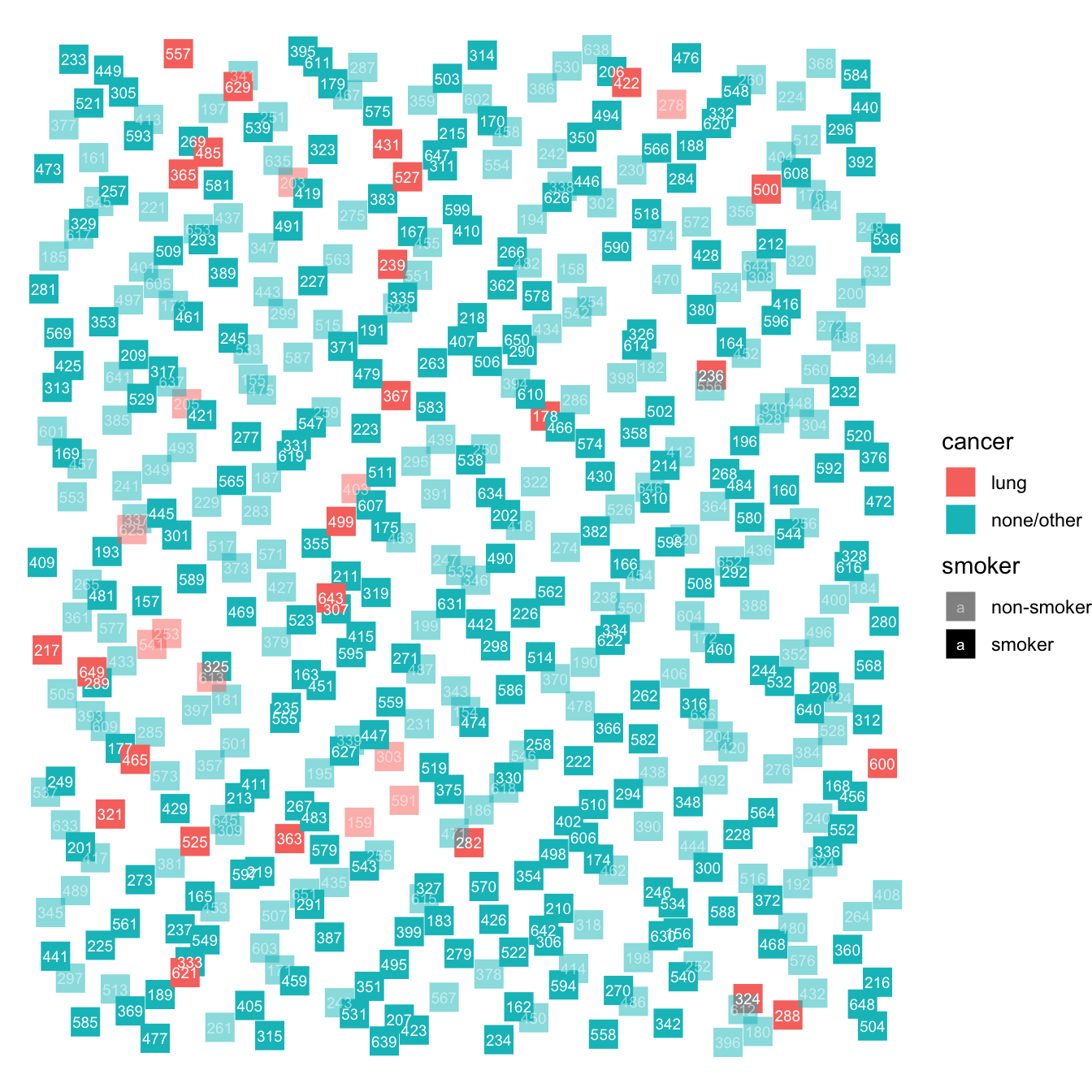
Figure 9.1: A schematic diagram showing the individuals in a hypothetical population, randomly placed in the field.
Person 217 is a smoker with lung cancer (smoker = opaque, lung cancer = red). Just below them is a non-smoker (transluscent) with lung cancer (red). But the large majority of the population does not have lung cancer. About half the population smokes.
It’s easier to see the relative proportions of each group if we re-arrange the individual blocks as in Figure 9.2. Doing this shows that the vast majority of people do not have lung cancer. For the people with lung cancer, somewhat more than half smoke, while for people without lung cancer
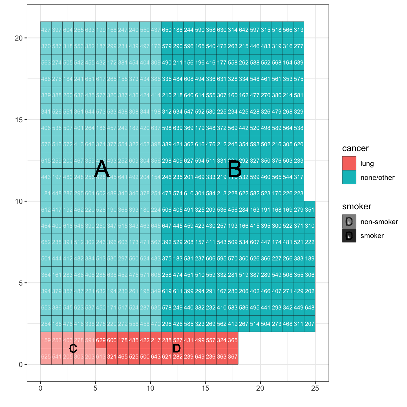
Figure 9.2: The population data arranged neatly into rows and columns so that it’s easy to see the relative size of four groups: A) non-smokers without cancer; B) smokers without cancer; C) non-smokers with lung cancer; D) smokers with lung cancer.
Table 9.1: The number of people in each of the four lettered groups in Figure 9.2.
| cancer | smoker | count | group_letter |
|---|---|---|---|
| none/other | non-smoker | 209 | A |
| none/other | smoker | 255 | B |
| lung | non-smoker | 11 | C |
| lung | smoker | 25 | D |
A simple stratification, smoker ~ cancer, shows that smoking is somewhat more common Among the 11 + 25 people with lung cancer, 25 smoke, a rate of 69%. Compare this to the 209 + 255 people without lung cancer: the smoking rate is 255/464, or 45%. (See Table 9.2.)
Table 9.2: Stratifying smoking by cancer: smoker ~ cancer.
| non-smoker | smoker | |
|---|---|---|
| lung | 0.05 | 0.09 |
| none/other | 0.95 | 0.91 |
Since the interest is whether smoking causes cancer (and not whether cancer causes smoking), it’s more natural to carry out the stratification in the other direction, cancer ~ smoking, as in Table 9.3.
Table 9.3: Stratification of cancer by smoking: cancer ~ smoker
| lung | none/other | |
|---|---|---|
| non-smoker | 0.31 | 0.45 |
| smoker | 0.69 | 0.55 |
Table 9.3 shows something much more sinister than Table 9.2, even though both tables are based on the same data. In Table 9.2, smoking is about 50% more prevalent among those with lung cancer than those without. But in Table 9.3, lung cancer is 80% more common among smokers than non-smokers. (Keep in mind that this is simulated data. We’ll get to the real data in a moment.) Both tables are faithful to the data, but the two different stratifications – cancer ~ smoker as opposed to smoker ~ cancer – provide different information.
cancer ~ smoker: What’s the risk that someone who smokes will get lung cancer compared to the risk for a non-smoker?smoker ~ cancer: For someone with cancer, what’s the risk that they will smoke, compared to someone without cancer?
The public health issue is, of course, whether smoking should be discouraged in order to reduce the risk of lung cancer. The information from cancer ~ smoker is informative to someone contemplating whether to stop smoke. Perhaps it’s easiest to think about the difference between smoker ~ cancer and cancer ~ smoking using the concept of causality. We’re concerned whether smoking causes cancer; smoking is the explanatory factor while cancer is the possible response.
Let’s turn from simulated data to the actual data available in 1950. Recall that there was no systematic database of cancers and smoking. There was little if any funding to support research about cancer and smoking, so any data collection effort would necessarily be small in scale.
In the 1940s, Dr. Lyle Baker was an oncologist at the Veteran’s Administration hospital in Hines, Illinois. As reported in Schrek et al. (1950):
In 1941, Dr. Baker started the practice at this hospital of having a clerk take a history of the smoking habits of each patient at time of admission by means of a questionaire…. In 1948, Drs. Ballard and Dolgoff summarized 5,003 records, selected at random, as to such factors as smoking habits and diagnosis. These men were particularly interested in the relation of smoking with peptic ulcer and heart disease. The data thus obtained were coded and placed on punch cards to facilitate analysis. The punch cards were prepared and handled by Mr. Vernon Graunke and Mr. G.O. Baldo, of Veterans Administration. The 5,003 records are reviewed in this paper to determine the association of smoking and cancer.
This is a case-control study, so named because many of the people involved are identified specifically because they are cases of lung cancer, while the remaining people – the “controls” – are people without lung cancer.
There’s good reason to think that the cases in the case-control data are representative of that part of the population with lung cancer. But there is no reason to think that the smokers in the case control data are representative of the population of smokers. Figure 9.3 shows simulated case-control data. Note that among smokers (groups B and D) more than half have lung cancer, dramatically larger than in the population.
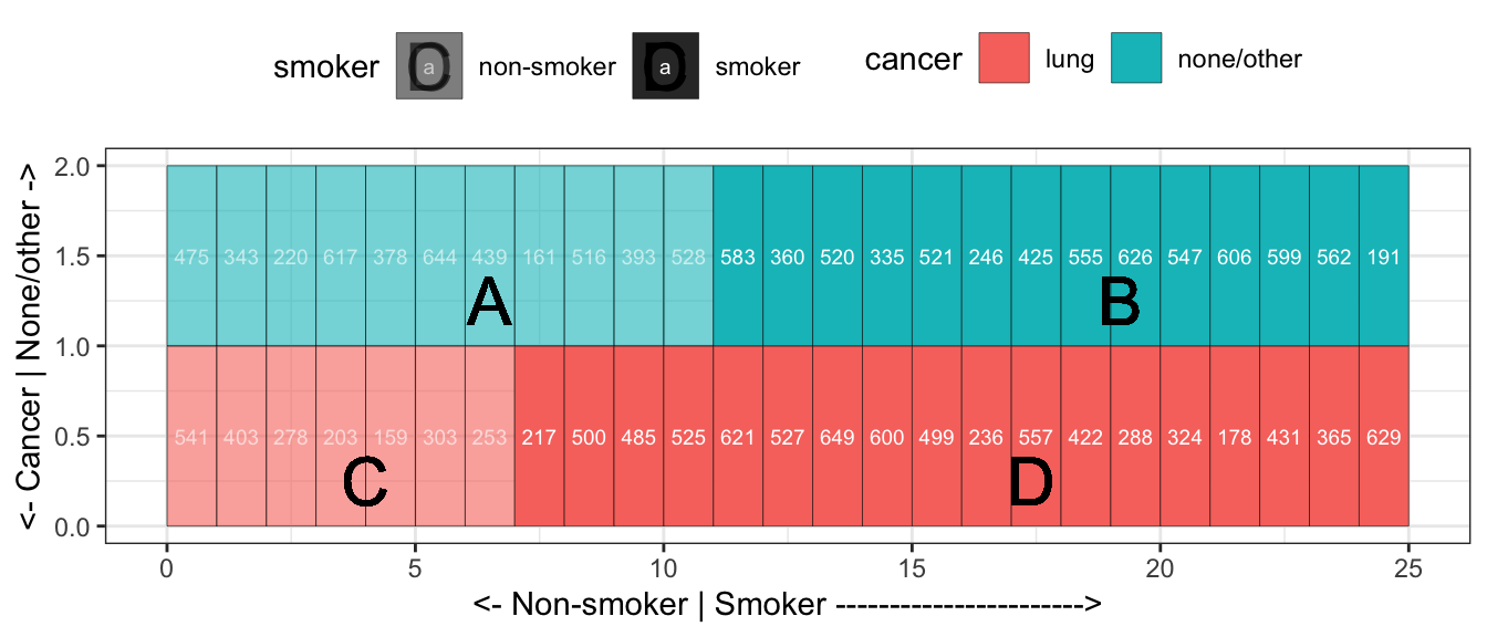
Figure 9.3: Cases and controls. While the cases are a small fraction of the population, they constitute about half of the case-control data.
Because the smokers in the case-control data are unrepresentative of the broader population, the stratification cancer ~ smoker need not give an accurate description of the population. On the other hand, since the cases in the case-control data are representative of people with lung cancer, the stratification smoker ~ cancer will give an accurate description.
Regretably, the question of interest, cancer ~ smoker, is not the question we can directly answer with case-control data. So, we are forced to work with an accurate answer to a question which is not directly meaningful: smoker ~ cancer.
In the 1940s case-control data reported in Schrek et al. (1950), focussing on men in their forties, 77% of the men with lung cancer smoked versus 58% smoking in the group who did not have lung cancer.
Looking at those two rates – 77% and 58% – may give you some impression about the extent to which smokers are at a higher risk of lung cancer, but will not directly answer the question. To help you understand the importance of the technique described in the next section, I ask you to use your intuition applied to the 77% versus 58%. Looking at those two numbers, to what extent is smoking associated with a higher rate of lung cancer? Choose one of these possibilities:
- The numbers say nothing, the risk is about the same in the two groups.
- There is little relationship, the risk is about 20% bigger among the smokers.
- There is a moderate relationship, the risk is about 50% bigger among the smokers.
- There is a strong relationship, the risk is about 100% bigger among the smokers.
- The risk is bigger still.
9.2 Inverse probability and Bayes’ Rule
Now let’s sort out what the relationship really is. Referring to Figures 9.2 (the population) and 9.3 (the case-control data) we can calculate some proportions in terms of the marked areas A, B, C, and D. For example:
- Case-control data gets it right:
- Proportion of cancer cases who smoke: p(Smoker given cancer) = D / (C + D) = 77%
- Proportion of non-cancer cases who smoke: p(Smoker given non-cancer) = B / (A + B) = 58%
- Case-control data is potentially misleading:
- Proportions of interest
- Proportion of smokers who have cancer: p(Cancer given smoker) = D / (B + D)
- Proportion of non-smokers how have cancer: p(Cancer given non-smoker) = C / (A + C)
- Other proportions we can calculate:
- Proportion of smokers: p(Smoker) = (B + D) / (A + B + C + D)
- Proportion of non-smokers: p(Non-smoker) = (A + C) / (A + B + C + D)
- Proportion of cancer cases: p(Cancer) = (C + D) / (A + B + C + D)
- Proportion of non-cancer cases: p(Non-cancer) = (A + B) / (A + B + C + D)
- Proportions of interest
Confirm to yourself that each of these eight proportions are what they claim to be.
The two proportions we want to compare are
\[\mbox{p(Cancer given smoker)} = \frac{D}{B + D}\] and
\[\mbox{p(Cancer given non-smoker)} = \frac{C}{A + C}.\]
We can’t accurately estimate these quantities directly from the case-control data, but as a matter of arithmetic, we can find each of them by multiplying three quantities together:
\[\frac{D}{B + D} = \frac{D}{C + D} \cdot \frac{C + D}{A + B + C + D} \cdot \frac{A+B+C+D}{B+D}\]
\[\frac{C}{A + C} = \frac{C}{C+D} \cdot \frac{C + D}{A+B+C+D} \cdot \frac{A+B+C+D}{A + C}\]
You can see that the equations are correct by cancelling out the corresponding numerators and denominators.
Looking up descriptions behind the various quantities, we get
\[\mbox{p(Cancer given smoker)} = \frac{\mbox{p(Smoker given cancer) p(Cancer)}}{\mbox{ p(Smoker)}}\] and
\[\mbox{p(Cancer given non-smoker)} = \frac{\mbox{p(Non-smoker given cancer) p(Cancer)}}{\mbox{ p(Non-smoker)}}\]
These arithmetic relationships are instances of Bayes’ Rule. The calculation of a proportion like p(Cancer given smoker) from an inverted proportion, p(Smoker given cancer), is called inverse probability or Bayesian statistics.
The case-control data, even though it’s not representative of the overall population, gives us a good estimate of p(Smoker given cancer) and p(Non-smoker given cancer). The case control data does not give good estimates of p(Cancer) or p(Smoker) or p(Non-smoker).
A nice feature of Bayes’ Rule is that p(Cancer) and p(Smoker) are relatively easy to estimate from sources other than the case-control data. Comparing hospital admissions data to population estimates gives p(Cancer). A survey of a sample of the population gives p(Smoker). So, evenTo illustrate, suppose we find out from national sources that about 60% of men in their forties are smokers (in the 1940s), and that 0.25% of men in their forties have lung cancer. Plugging these proportions into Bayes’ Rule gives:
\[\mbox{p(Cancer given smoker)} = 0.77 * 0.025 / 0.55 = 3.2\%\] and \[\mbox{p(Cancer given non-smoker)} = 0.23 * 0.025 / 0.45 = 1.4\%\]
In other words, the case-control data (combined with other knowledge about the population) shows that lung cancer is more than twice as common among smokers than non-smokers. The data here are from the 1940s and 1950s. Subsequent research has shown that smokers have much greater than twice the risk of lung cancer compared to non-smokers.
9.3 Which population?
Data scientists often work with large data sets. There’s a temptation to think that the size of the data set justifies treating the data as a representative sample from the population of interest. As we’ll discuss later in Chapter ??, you need to be cautious about this and look in detail at the factors determining which observations made it into the data.
In the previous sections of this chapter, we’ve discussed using the arithmetic of Bayes’ Rule to correct for deficiencies in data. The case-control cancer/smoking data introduced one such deficiency: the data had large proportion of cancer cases unrepresentative of the population as a whole.
But even when you have a representative sample, you need to be aware of the ways that it may not be directly suitable for estimating the quantity of interest. To illustrate, consider our finding that, in men in their forties, lung cancer in 1940 was more than twice as common among smokers than non-smokers. That is true, but doesn’t directly address the question of interest: What is the risk of getting lung cancer for smokers compared to non-smokers?
The problem is that the case-control data provided a snapshot: people who have a diagnosis of lung cancer compared to others. But the risk of interest is that of getting lung cancer, not having lung cancer. The proportion of the population diagnosed with lung cancer is in reality a severe under-estimate of the risk of getting lung cancer. Why? Because only a small fraction of people who will get lung cancer currently have it. Most will develop it later.
The risk of having a disease is called the prevalence of the disease. The risk of getting a disease in a specified interval of time is called the incidence. Recent data indicates that the lung-cancer incidence for 45 year-old men over the next ten years is eight times higher for current smokers than for never smokers. (Woloshin et alia 2008) The lifetime risk of lung cancer for smokers is about 15% compared to about 2% for those who have never smoked. (Bruder et al. 2018)
We’ll return to some of the challenges of presenting risk in an informative way in Chapter @ref(communicating_about_risk).
9.4 Exercises
rrr etude_list(Bayes_exercises)
References
Bruder, C., J. L. Bulliard, S. Germann, I. Konzelmann, M. Bochud, and A Leyvraz M.and Chiolero. 2018. “Estimating Lifetime and 10-Year Risk of Lung Cancer.” Preventive Medicine Reports 11: 125–30. https://doi.org/doi:10.1016/j.pmedr.2018.06.010.
Schrek, Robert, Lyle A. Baker, George P. Ballard, and Sidney Dolgoff. 1950. “Tobacco Smoking as an Etiologic Factor in Disease. I. Cancer.” Cancer Research 10: 49–58.
Woloshin et alia, Steven. 2008. “The Risk of Death by Age, Sex, and Smoking Status in the United States: Putting Health Risks in Context.” Journal of the National Cancer Institute 100 (12): 845–53. https://www.ncbi.nlm.nih.gov/pmc/articles/PMC3298961/.