Chapter 15 Sampling variation

15.1 Our approach to sampling variability

We will use a simulation technique to explore sampling variability. In the simulation we’ll imagine that we have a census of a population in the form of a data frame. Given this data frame, a computer can easily select a set of random rows to constitute a sample. Then, we’ll do some statistical work – say, training a model and calculating an effect size – using that random sample. We’ll use the phrase sampling trial to describe this process of pulling out random rows to be our sample and doing some statistical work.

By conducting many sampling trials and collecting the result of the statistical work from each, we’ll be able to construct a new data frame where the unit of observation is a trial. Examining variability from trial to trial, for instance by constructing a 95% coverage interval, will provide the quantification of the amount of variation due to sampling.

For the purpose of illustration, we’ll use as the simulated census a data frame containing 8636 rows about runners in a 10-mile race. Experience and mathematical theory show that the patterns that will be displayed here using the 10-mile race data appear generally in data of all sorts.

As an example, we’ll draw a random sample of size n = 400 from the population of runners. The statistical work will be to build a function of running time versus age and sex based on the ten-mile-race data. Figure 15.1 shows one trial in the form of a graph of the function.

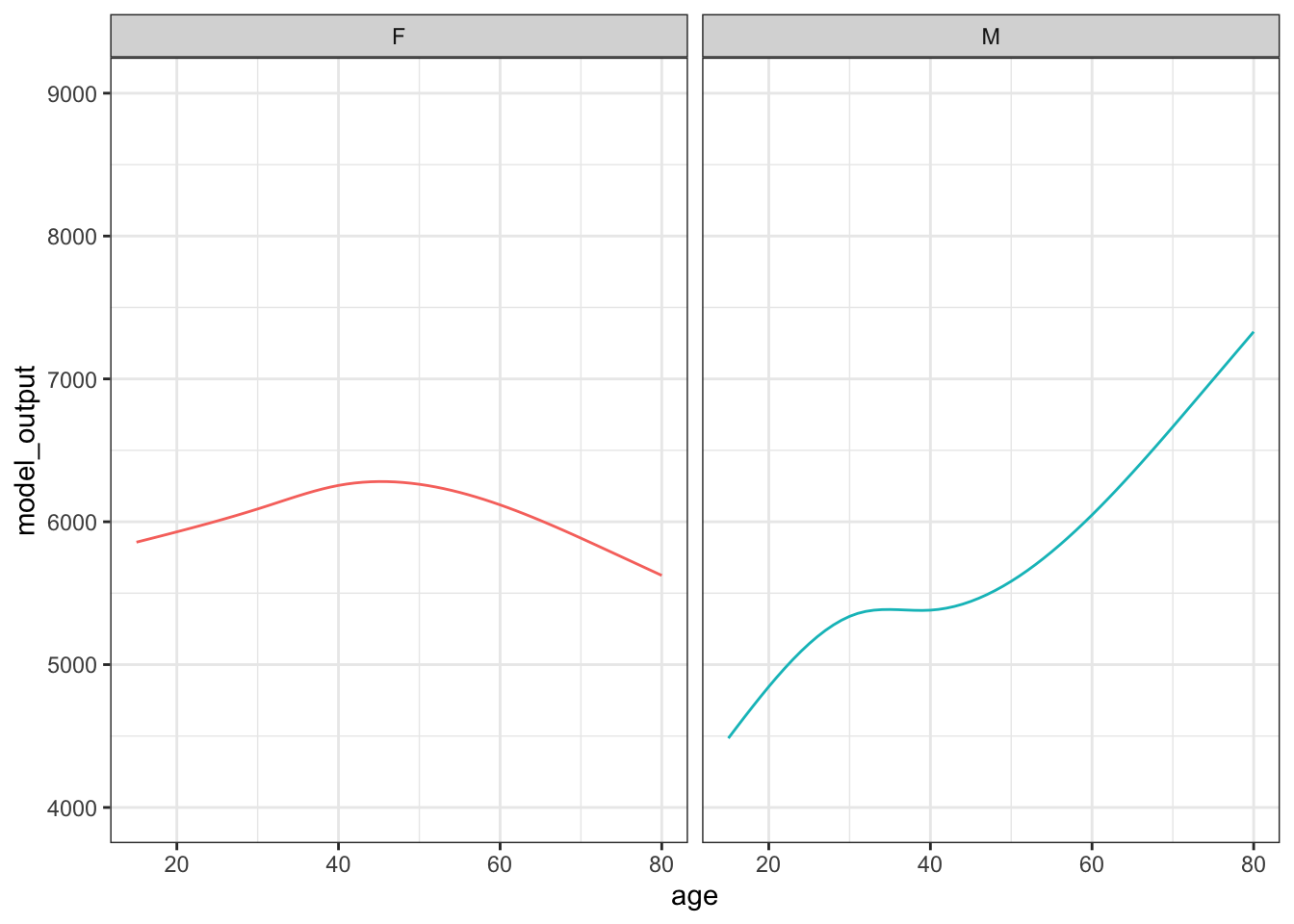
Figure 15.1: The results of one trial in which a simple random sample of size n = 400 was selected from the population and the data used to train a model of running time versus age and sex.

Figure 15.2 shows 10 sampling trials.

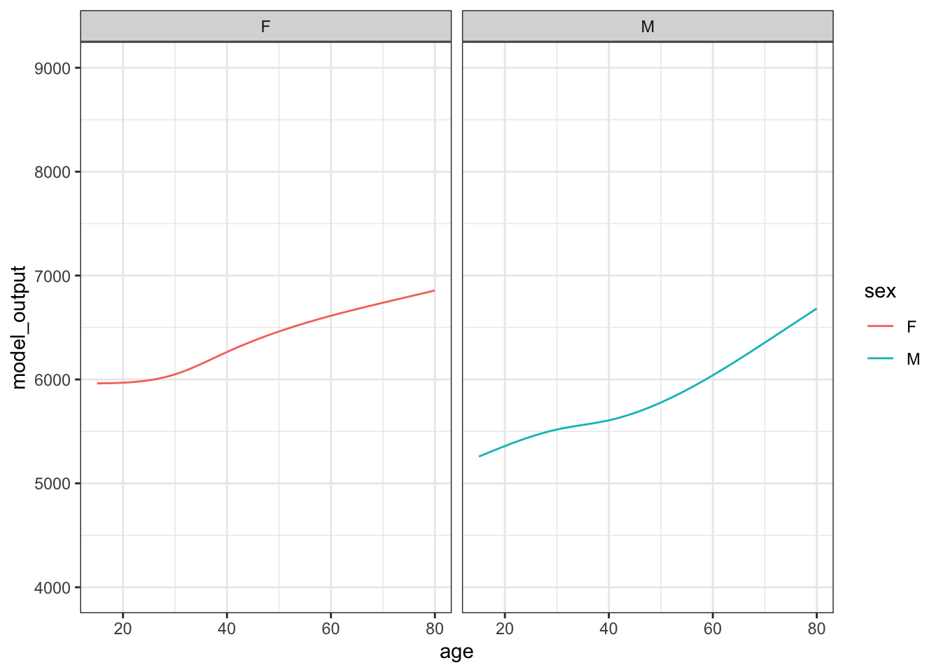
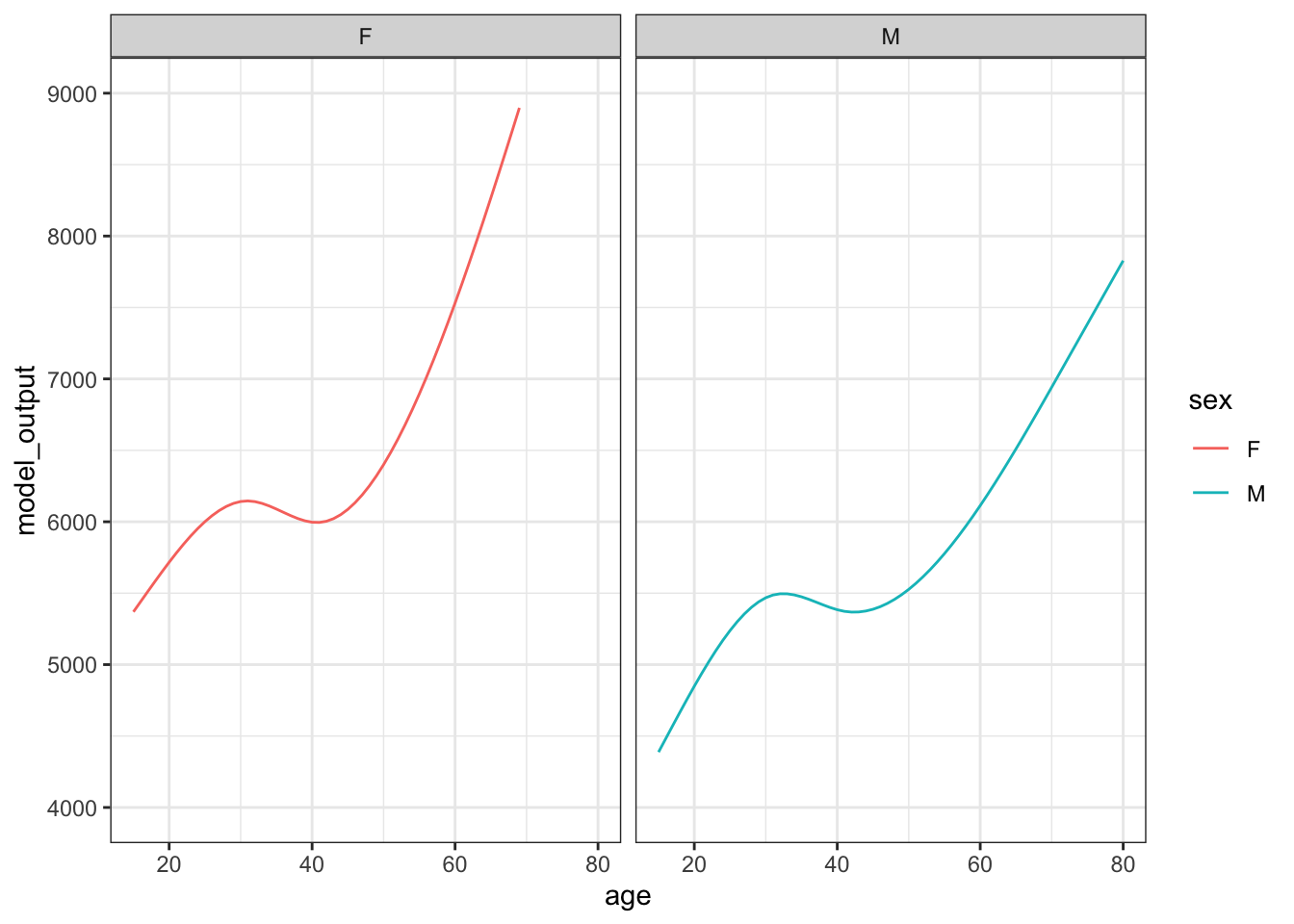
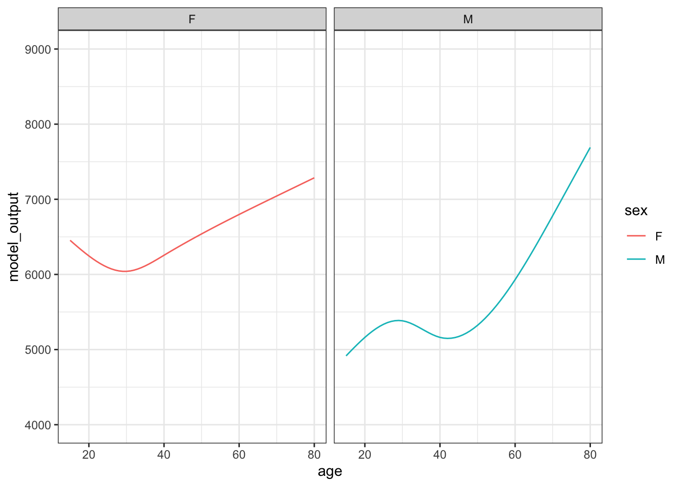
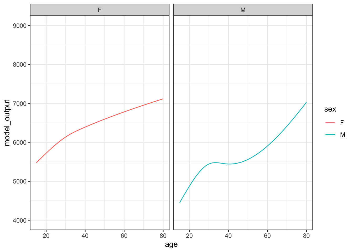
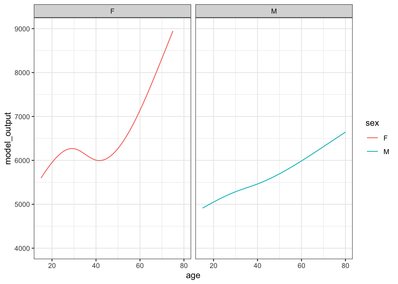
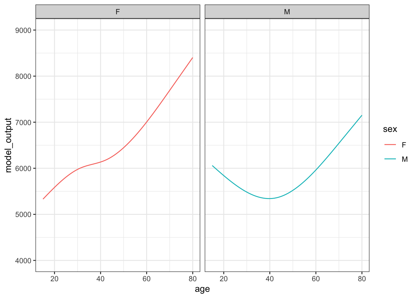
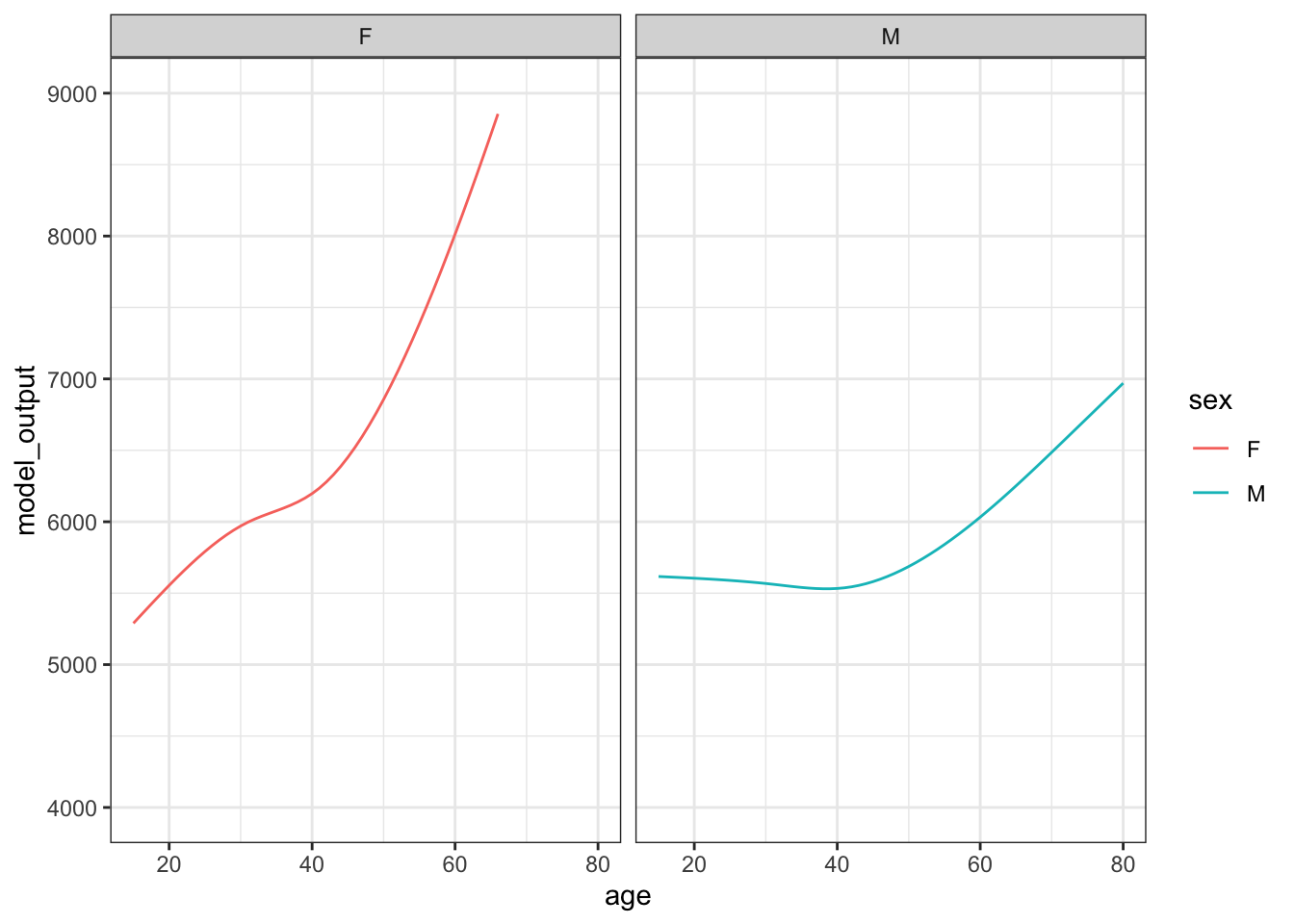
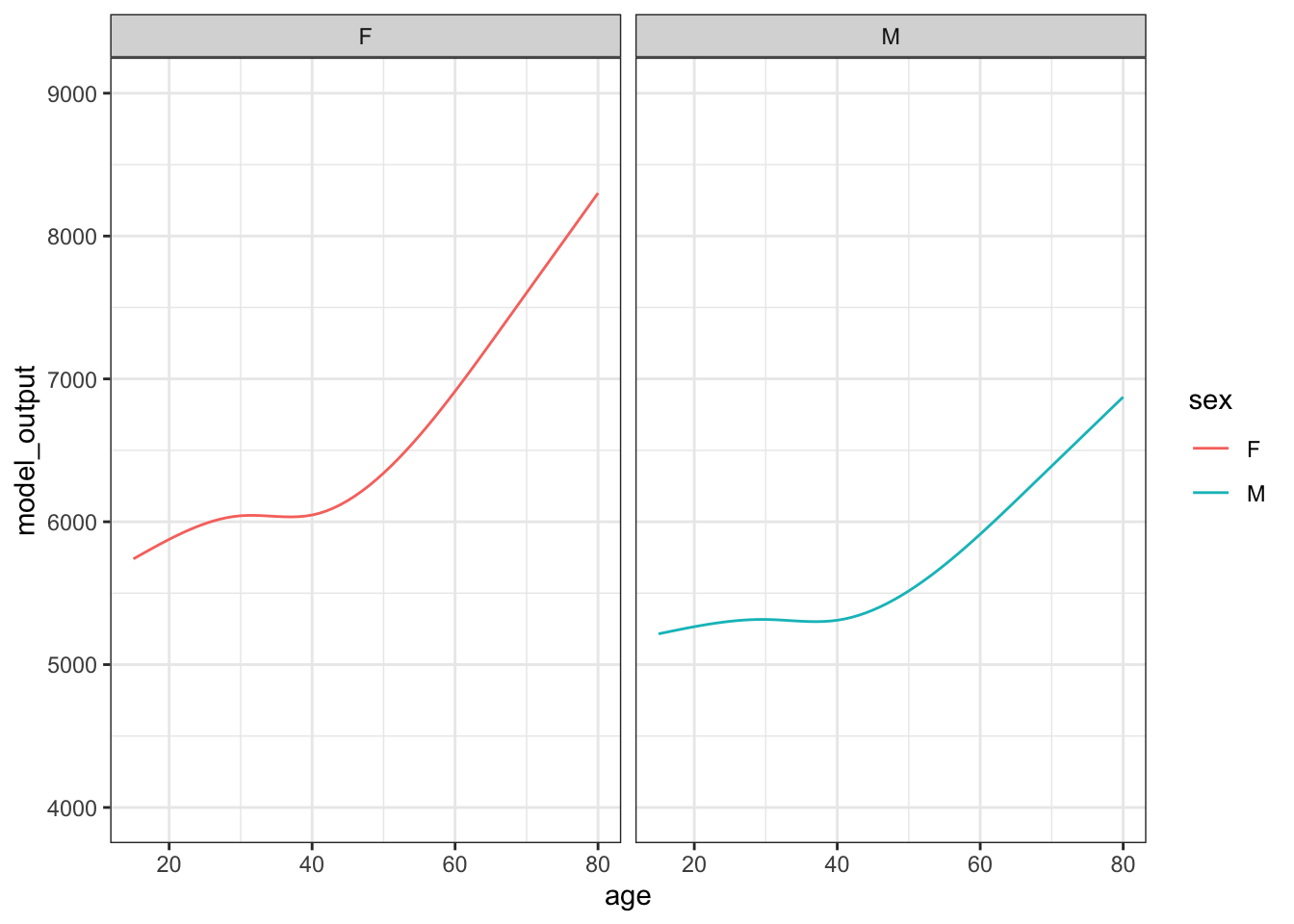
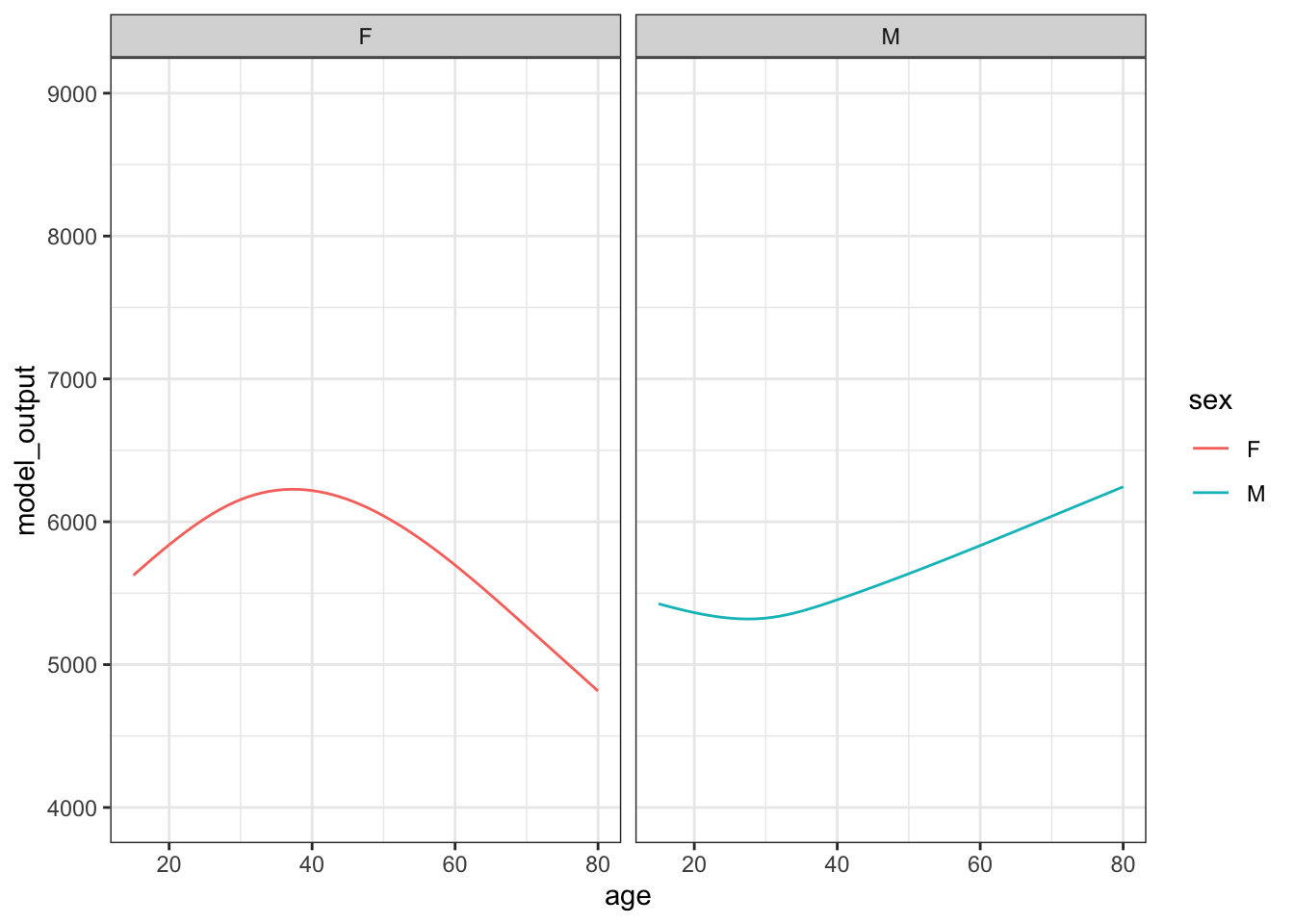
Figure 15.2: The results from ten sampling trials each consisting if drawing a sample of size n = 400 from the runner population and training a model of running time versus age and sex.

Each sampling trial produces a somewhat different function. From age 30 to 50 the functions are all about the same. The functions fan out for ages under 25 and over 60, telling us that the data are not very informative for these ages about how running time changes with age.

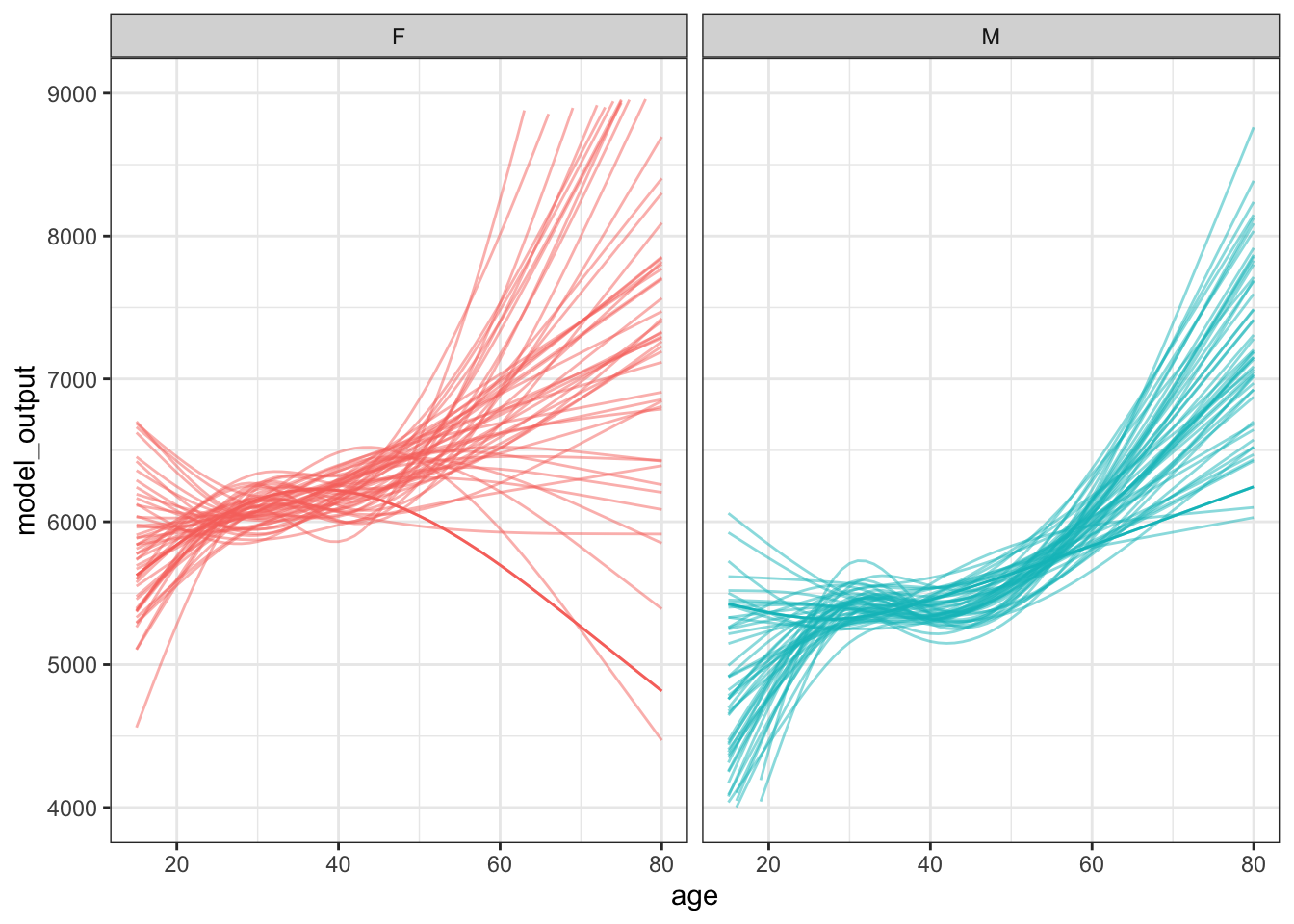
To display the sampling variability more clearly, run more trials and present the results all in the same graphics frame, as in Figure 15.3.

Figure 15.3: 50 sampling trials in constructing flexible linear models time ~ age + sex using samples of n = 400 rows from the ten-mile-race data.

15.2 Confidence intervals

From each of the functions shown in 15.3 we might decide to calculate an effect size, for instance, how the running time varies with age. With practice, you can sometimes read this effect size directly off of the graph of the function. The effect size of age on running time is the slope of the function.

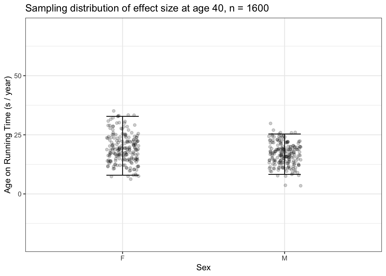
When the interest is in an effect size, it makes sense to include the effect size calculation directly in the statistical work being done in each sampling trial. To illustrate this, Figure ?? shows many sampling trials in which the model running time versus age and sex was trained and, from the model, the effect size of age on running time calculated for 40-year olds.

Figure 15.4: (ref:effect-variability-1-cap)

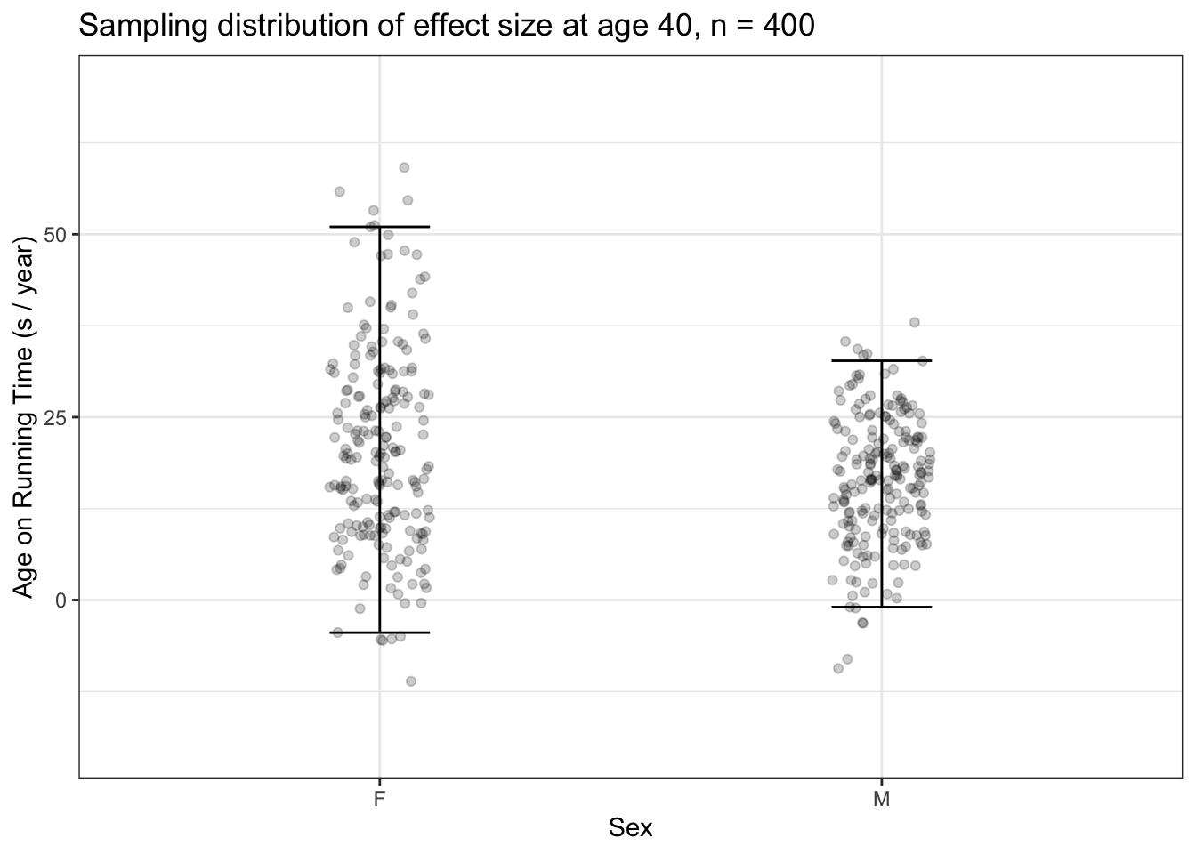
Examine Figure 15.4 carefully. First, note the graphics frame: The vertical axis is the effect size of age on running time, the horizontal axis is sex. Each dot is the outcome of one sampling trial. The vertical spread of dots shows the range of different results we might get from any particular trial. For instance, an effect size of 25 s/year1414 The effect size shows how running time changes with respect to the runner’s age. An effect size of 25 s/year indicates that, on average, runners slow down by 25 seconds per year of age. for men is a plausible outcome from one trial, but not an effect size of 50 seconds per year of age.

You can also see that there are plenty of trials for which the effect size for women is greater than men, and plenty of trials where the reverse is true. This means that a sample of size n = 400 is not a reliable way of finding a difference (if one exists) between women and men with respect to their change in running performance as they age.

The interval layer in Figure 15.4 is simply a way of summarizing the spread due to sampling variation. Following statistical convention, we’re using a 95% coverage interval as the summary.

There is a special name for this sort of interval on sampling trials: a confidence interval. This will take some getting used to. A confidence interval is a special sort of coverage interval. What makes the confidence interval special is that it is being calculated across sampling trials.

Confidence intervals play a very important role in interpreting effect sizes and other statistics. A confidence interval tells us the precision to which we know the effect size. When you are comparing two confidence intervals, as you can do for men and women in Figure ??, look at whether the intervals overlap. When they do overlap, there’s no statistical justification for a claim that the effect size differs between the two groups being compared.

15.3 Improving precision

As just mentioned, a confidence interval indicates the precision with which your data pin down an effect size (or whatever other statistic is being calculated in the sampling trial). The greater the precision, the more you are able to discern, say, the difference between two effect sizes.

How do you arrange to have greater precision? It turns out that the length of a confidence interval is shorter (that is, more precision) the larger is the sample size n. Indeed, there’s a more specific statement to be made: the length of a confidence interval is, roughly, proportional to \(1 / \sqrt(n)\). The confidence intervals in Figure 15.4 are based on sampling trials where each trial has n = 400. If we would like to have shorter confidence intervals, we need to collect more data. For instance, to get confidence intervals that are half as long as those in Figure 15.4, we would want to work with four times as much data, that is, a sample size of n = 1600.

Figure 15.5: 200 sampling trials for the effect size of age on running time, each trial with a sample of size n = 1600. The intervals shown here are roughly half as long as those seen in Figure 15.4, where n was 400.

15.4 Example: Over the hill?

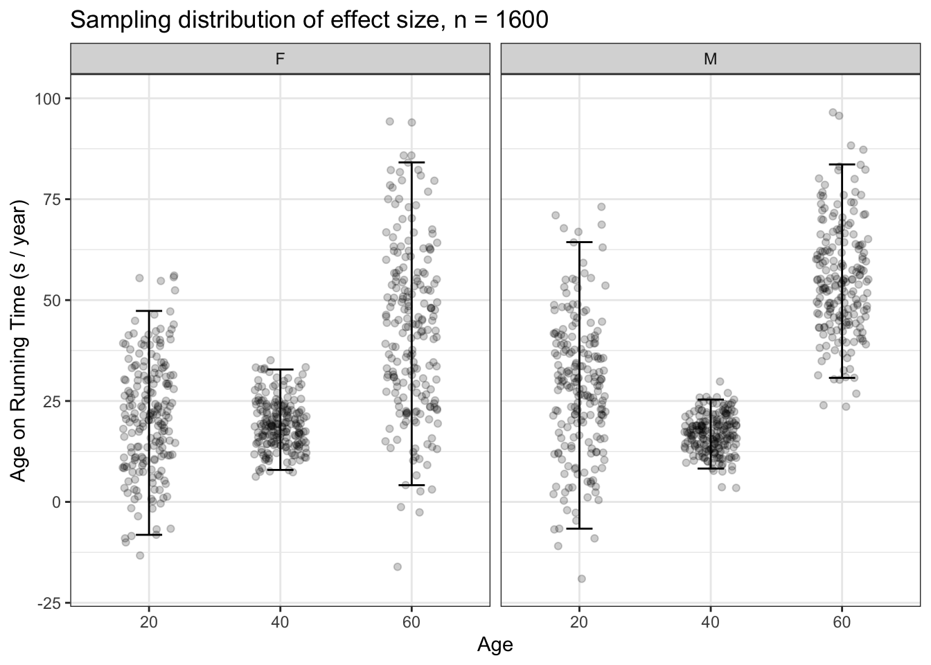
It’s conventional wisdom that athletes, once they reach a certain age, slow down faster. But do the data from the 10-mile race support this. Let’s calculate a confidence interval on the effect size of age on running time, looking at age 20, 40, and 60. The confidence intervals with n = 1600 (Figure 15.6)

Figure 15.6: 200 sampling trials with n = 1600 comparing the effect size of age on running time at ages 20, 40, and 60 years. The differences in effect size for men at age 40 and 60 are evident: the confidence intervals do not overlap.

15.5 Getting practical

The technique we’ve used in this chapter to demonstrate sampling variability is based on a simulation in which we pretend that our data is the population and make many sampling trials, with n smaller than the population, to see the extent of sampling variability.

As you’ve seen, the length of confidence intervals depends on n in a manner proportional to \(1 / \sqrt{n}\).

Wouldn’t it be nice to be able to use all our data for constructing confidence intervals. In the ten-mile race data, there are 8636 runners. Using n = 8636 would, in theory, produce confidence intervals less half as long as those seen in Figure 15.6, where \(n = 1600\).

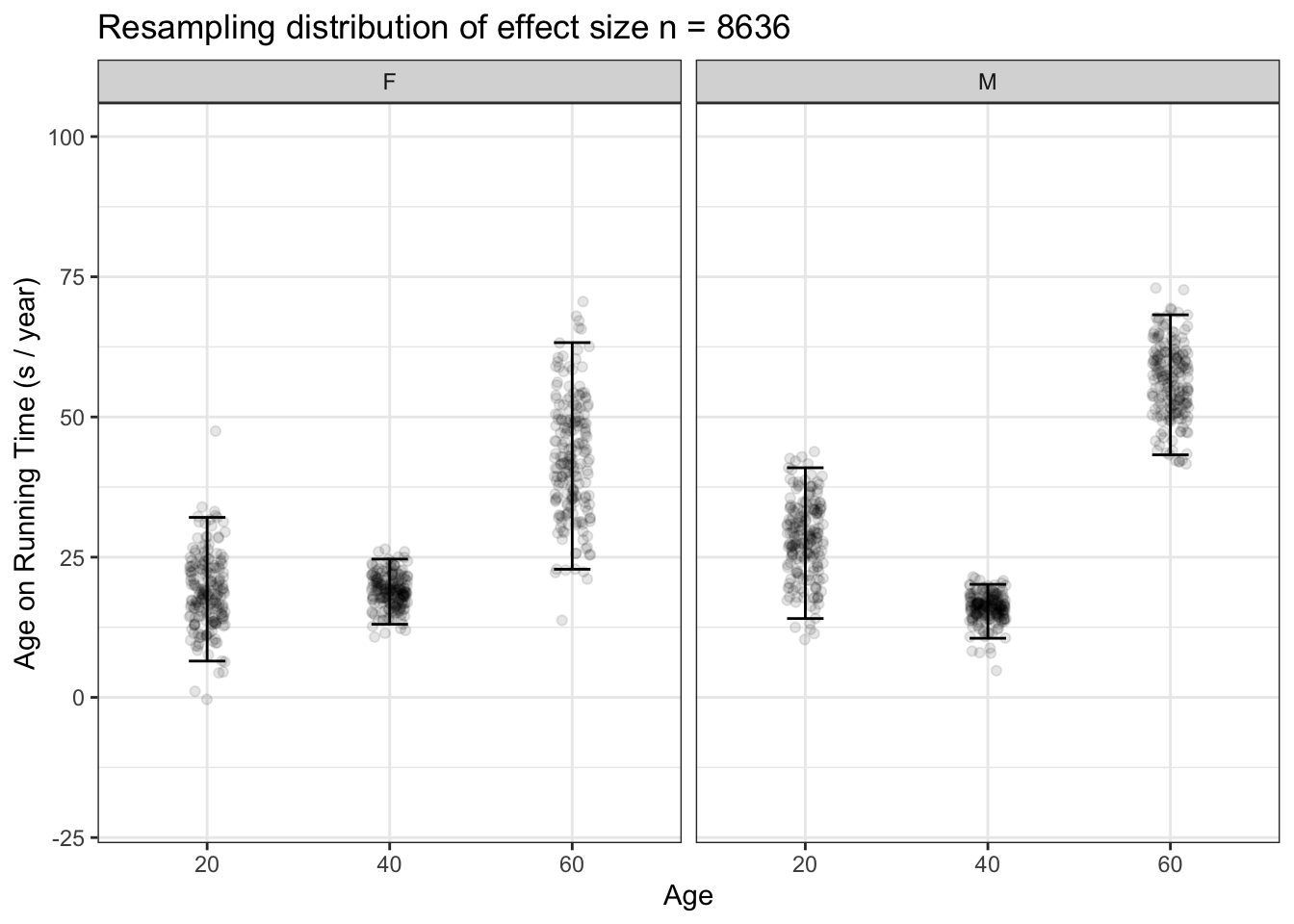
We can accomplish this by a very small change in method. Rather than setting as our hypothetical sample one copy of the ten-mile race data so that the population has 8636 rows, let’s duplicate it many times and create a simulated population that’s much, much larger than the actual data. If we used 100 duplications, we would have a popultion with 863,600 rows. With this very large population, we can easily draw samples of size n = 8636 and find the confidence intervals using all our data. Figure 15.7 shows the results of this method, which is called resampling.

Figure 15.7: 200 resampling trials with n = 8636, that is, the whole population, comparing the effect size of age on running time at ages 20, 40, and 60 years. The differences in effect size for men at age 40 and 60 are evident: the confidence intervals do not overlap.

We’ll consider resampling in more detail in the next chapter.

15.6 Three distinct intervals

Sampling distributions have been a subject of research in statistics for more than a century. Much is known about them from mathematical analysis of probabilities and from simulations such as the ones presented above. In particular, much is known about what determines the extent of spread of the sampling distributions. Regretably, it’s also known that the spread of sampling distributions is an intrinsically confusing concept to a person – perhaps you – encountering it for the first time.

Because it’s so easy to confuse the spread of a variable, the prediction interval from a model, and the sampling distribution of a statistic, we’re going to use specific and distinct terms for each.

• The coverage interval refers to the spread in a variable.
• The prediction interval refers to the spread in the possible actual outcomes that is anticipated when making a prediction.
• The confidence interval refers to a sampling distribution of a statistic such as an effect size.

Coverage intervals refer to data; they describe the variables themselves and are not related to any model. A prediction interval refers to an individual model; it describes the uncertainty in a prediction. A confidence interval also refers to a model. But it is not about the quality of predictions, it is about comparing different models to one another. So, two research groups who have made independent studies of the same issue can use the confidence intervals on their models to indicate whether their results are inconsistent with one another or whether the differences in their results are plausibly the result of sampling variation.

Each of these three intervals can be calculated at any percentage level: 50%, 90%, and so on. However, it’s the convention for all three intervals to use the 95% level. Research papers that use these interval should, ideally, say explicitly which level they are using. And, certainly, they should say explicitly if they are not using the 95% level.

But data science is important in large part because it’s results are used for making decisions. The people who make the decisions are often not specifically trained in statistics and they may not be at all aware of the somewhat subtle considerations that inform the use of 95% as a level. In communicating with such people, be aware that they may not correctly interpret an interval.

15.7 Example: Coverage, prediction, and confidence in running times

To help you see the differences among the coverage interval, the prediction interval, and the confidence interval, let’s put them side by side. The example will be based on the ten-mile-race data. We’ll look at two different models, time ~ age where the explanatory variable is quantitative and time ~ sex where the explanatory variable is categorical. The concepts apply equally well to models with more explanatory variables, but the graphic become too busy to be useful.

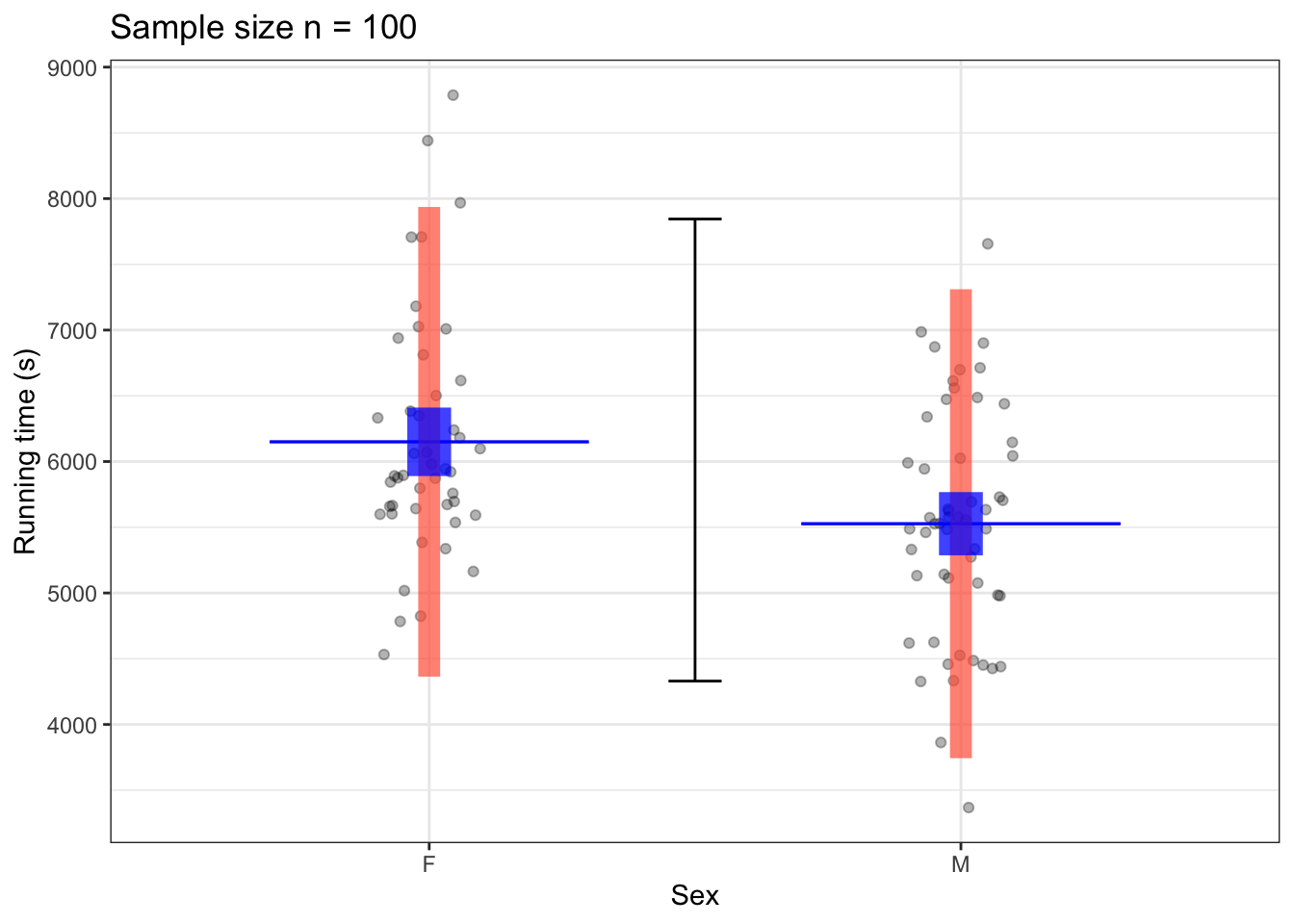
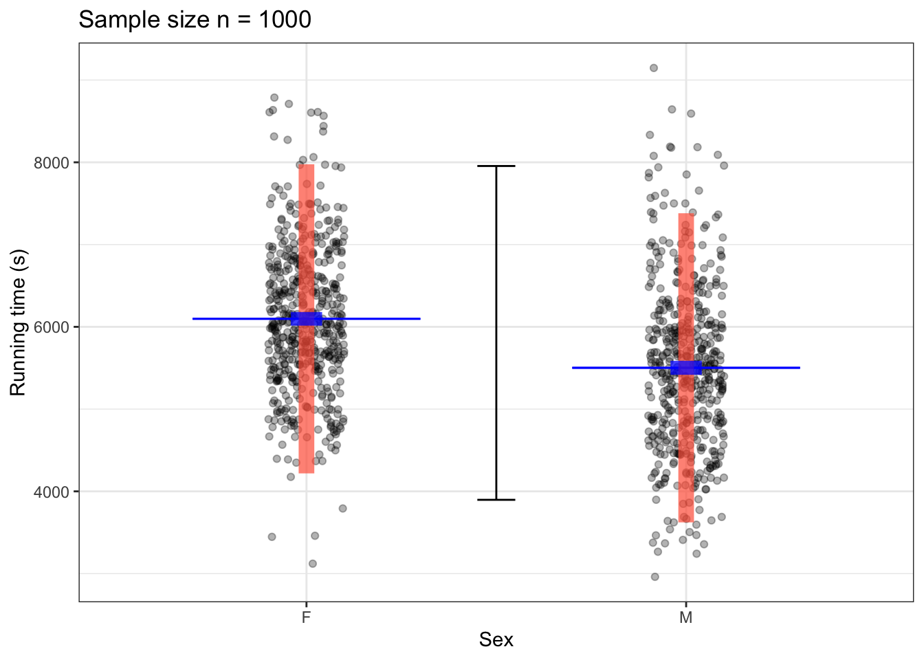
Figure 15.8: Coverage interval (black) for the variable time and prediction intervals (red bar), and confidence interval (blue bar) for the predictive model time ~ sex using samples of size n = 100 (left) and n = 1000 (right) from the TenMileRace data. The model output itself is shown as a thin blue line segment.

Figure 15.8 shows the 95% coverage interval for the variable time. Note that there is only one interval because coverage intervals are about a single variable, not a relationship between two variables. The prediction intervals include most of the data at each level of the explanatory variable. The prediction intervals are centered on the model values. The length of the interval is only slightly smaller for the n = 1000 sample than for the n = 100 sample.

The confidence intervals in Figure 15.8 are much narrower than the prediction intervals, and include only a small part of the data. The length of the confidence interval is much narrower for the n = 1000 sample than for the n = 100 sample. According to theory, the bigger sample (with 10 times as much data) should have an confidence interval that is \(1 / \sqrt{10} \approx 0.32\) as long as the smaller sample.

Note that at either sample size, the coverage intervals for men and women do not overlap. This indicates that there is good evidence that the mean running times for men and women differ. On the other hand, the prediction intervals overlap substantially. This indicates (as is obvious from the raw data) that even if the mean time for women is longer than the mean time for men, there are plenty of individual women who are running faster than plenty of individual men.

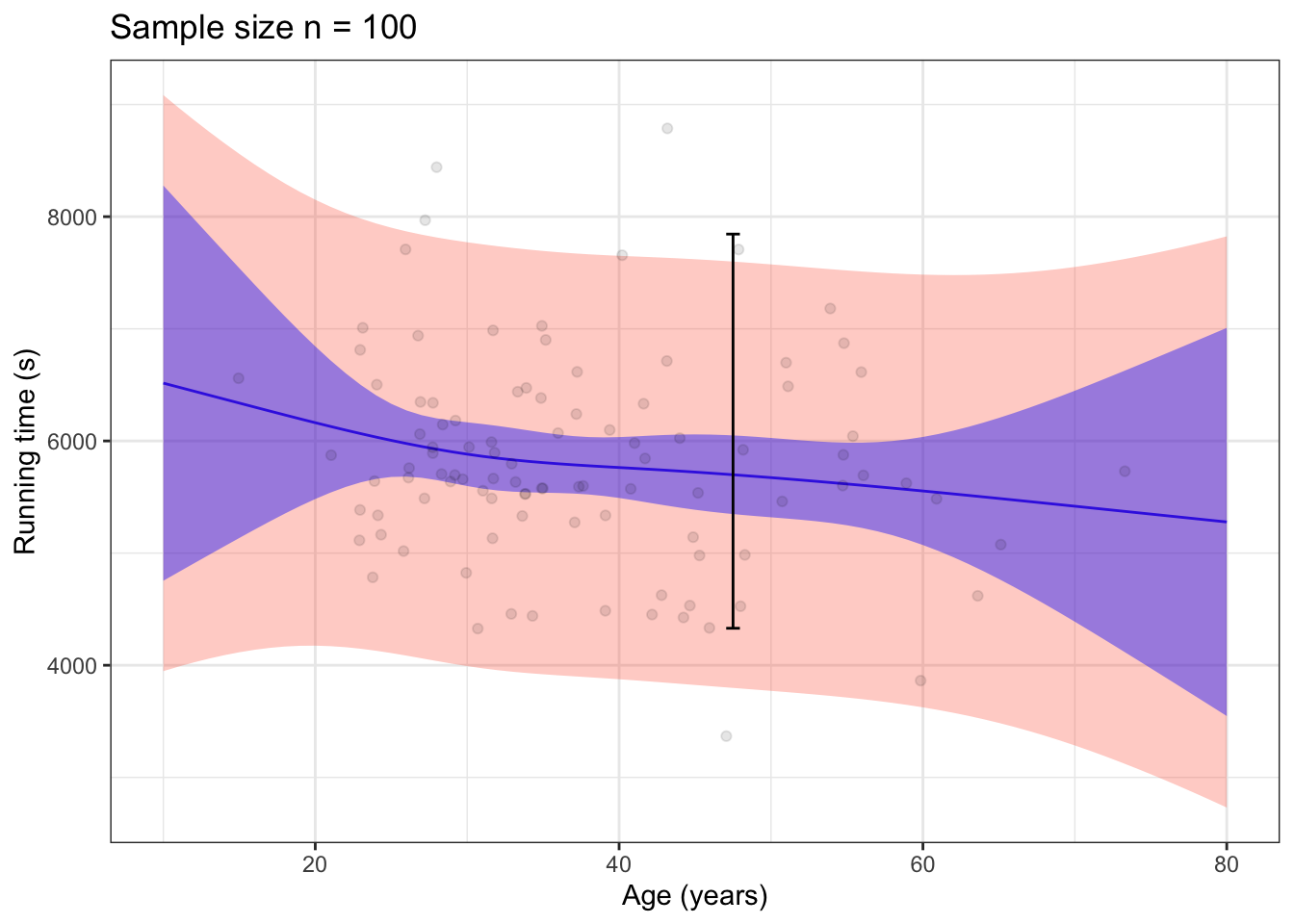
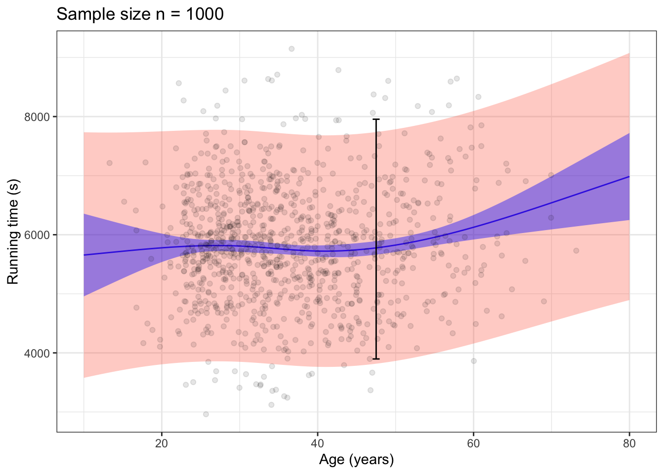
Figure 15.9: 95% prediction (red) and confidence (blue) bands for the model time ~ age for a sample size of n = 100 (left) and n = 1000 (right). The coverage interval for the variable time is drawn in black.

Confidence and prediction intervals can also be drawn for models with quantitative explanatory variables. Figure 15.9 shows the intervals for a flexible linear model time ~ age. Since there is an interval for any model input, confidence and prediction are drawn with bands. The top to bottom interval at any given input is the interval for that input. The bands show all of the intervals simultaneously.

The 95% prediction band covers almost all of the data. In contrast, the 95% confidence band is much narrower and depends on the sample size in the usual \(1 / \sqrt{n}\) fashion. The two-headed trumpet shape of the confidence bands reflect the additional uncertainty created when evaluating the model for extreme inputs where there is little or no data.

15.8 Confidence intervals and sample size

You have a data frame with n rows. You pick one of the variables and calculate a coverage interval.

Your colleague has access to a much larger data frame with 100n rows. How will her coverage interval differ from yours? The answer is that there is no systematic relationship between the size of the sample and the coverage interval of a variable.

Now a different question. You and your colleague each construct similar models based on the data, you with the n rows and your colleague with 100n rows. You each produce a confidence interval on a statistic, say, the model output when the inputs are at some specified value. How will your confidence interval differ from that of your colleague?

Here the answer is different. Your colleague’s interval, being based on 100 times as much data, will be 10 times narrower than your confidence interval. This is the sense in which more data leads to less uncertainty: the sampling distribution with a large sample will be narrower than with a small sample.

The width of a confidence interval depends systematically on the amount of data used in calculating the statistic. The general pattern is that more data leads to narrower intervals and, more specifically, that the width of the interval tends to be proportional to \(1 / \sqrt{n}\).

Finally, consider the prediction interval. A prediction interval is made up of two components: a part proportional to the model error and a part proportional to the confidence interval. The model error is about how close individual rows of the data frame are to the pattern described by the model. This is what the root mean square error is about: how close is the response variable value for a “typical” row to the output of the model when the inputs are at the explanatory variable values for that row. At any large sample size where the width of the confidence interval is much smaller than the RMSE error, the RMSE error does not depend systematically on the sample size.

The differing relationships between the coverage, prediction, and confidence intervals and the sample size is important for data science and statistics generally.

In large scale data science problems, often there is some readily accessible data that has a moderate size and a much larger set of data that can be accessed with special computing techniques from huge databases. The readily accessible data might take the form of a file that fits on your computer, whereas the huge database may span many computers in the cloud.

It’s a good practice to start with readily accessible data, displaying the data graphically, building predictive models, and so on. You can calculate prediction and confidence intervals using the readily accessible data. Those intervals might be so large that you can’t draw a useful conclusion. But often, the intervals are narrow enough that you can draw a conclusion or use the data to make a good decision. If so, there’s little benefit in carrying out the work again using the huge database. You already have what you need. (But do make sure that the accessible data is genuinely representative of the huge data, as would be the case if you sampled randomly from the huge data to create the accessible data.)

If the intervals are too wide to serve your purposes, figure out what width would let you make meaningful conclusions and decisions. Suppose, for instance, that the interval you get from the accessible data is ± 50 and you believe that your purpose requires an interval of ± 10. This gives you important guidance about your next steps. Since your current interval is five times wider than the one you need, you will want to access more data in order to produce smaller intervals. Your interval is five times as large as you need, so you will need about 25 times as much data to produce the small-enough intervals. (Remember, the width of a confidence interval is proportional to \(1 / \sqrt{n}\), so twenty-five times as much data will produce an interval that is one fifth the size of the original interval.)

For generations, a central problem in statistics was the scarcity of data. Statisticians were very careful to understand how much data is needed to justify a statement. Having more data meant that statements could be more strongly justified. More was better.

The methods developed by statisticians are still important. They provide the means to know how well a conclusion is justified by the data. But with very large data sets it can happen that a useful conclusion can be drawn with a small fraction of the data. In such situations, there’s little benefit to getting even more data.

15.9 A variety of vocabulary

For decades, statistics has been introduced in a manner that emphasized formulas for computing confidence intervals and such. In this book, as I think appropriate for a world of data science, such formulas and other techniques are incorporated into software. Rather than learning to repeat by hand the calculations already in software, we can take advantage of the software’s existence to focus our attention on the what and why of statistical quantities: how to use and interpret them rather than perform the calculations.

Software has been available for about 50 years. Before that, in the days before electronic computers were readily available, statisticians necessarily had to do the calculations themselves. In sophisticated statistical organizations, mechanical calculators were available for doing arithmetic, square roots, and such. And, often, these organizations had staffs of clerks who carried out the extensive calculations. (The clerks were called “computers”: people who compute.)

In doing the calculations, there are many intermediate steps that produce numbers to be used again later in the overall process. In order to keep the process orderly, it was useful to give names to these intermediate results. With experience, people learned to judge from the intermediate results what the final results would be. Consequently, the intermediate results were often presented in place of the final results.

To illustrate, consider the calculation of a confidence interval on the mean of some variable x. With software, we’re presenting confidence intervals as the values of the top and bottom of the intervals. Here’s how the calculation itself goes, with names of the results shown in bold letters.

1. Add up all the values of the variable x in your data and divide by the number of rows, n. This gives the sample mean of the variable.
2. Look again at the values of the variable x, but subtract from each of them the value of the sample mean calculated in step (1). These are the deviations, which you can think of as the prediction errors for the no-input prediction model. Another name used is residuals.
3. Square the residuals, add them up, and divide by n - 1. This gives the variance of the residuals.
4. Take the square root of the variance, producing the standard deviation of the residuals. (Think of “standard” as meaning “typical.”)
5. Multiply the standard deviation of the residuals by \(1 / sqrt{n}\). This new quantity is the standard error.
6. Multiply the standard error by 2, producing the 95% margin of error. Strictly speaking, the number is not exactly 2, but is the result of a separate complicated calculation, often done with printed tables to make it manageable, and which in the end results in a number very near 2. (Those tables contain critical values of the t distribution for many different values of n - 1, which is called the degrees of freedom.) The number you pull from the printed tables has its own name, t-star. (This is to be distinguished from a very similar table that gives z-star, which is used in calculations such as the confidence interval on the proportion.) And, in case you want to use some level other than the conventional 95%, the level has its own name: the confidence level.
7. Finally, to arrive at the confidence interval, calculate the top of the interval as the mean plus the margin of error and the bottom of the interval as the mean minus the margin of error. Alternatively, one can skip the addition/subtraction and write down the confidence interval immediately as mean ± margin of error.

It is, of course, challenging to learn this vocabulary. Is it necessary if you’re not carrying out calculations by hand? The bottom line of the calculations is the confidence interval, so that’s an important concept to master. As for the others, it’s nice to be aware of them, just as you’re aware that Sneezy is one of the Seven Dwarfs and Prancer is one of Santa’s reindeer.