Chapter 2 Data and information
(ref:chapter-tidy_data) Chapter 2
Data takes many forms, but all of them are records of observed facts. A list of countries and national capitals is data. A diary is data where the “facts” are your impressions and beliefs at the time you write them down. A policeman’s radar reading of a car’s highway speed is data, as are the locations, altitudes, speeds, and directions of the planes being tracked by an air-traffic control system. Data doesn’t have to be “correct”. The policeman’s radar reading might be distorted by reflections from the truck approaching in your rear-view mirror. Wikipedia is data even though the “facts” in some cases do not necessarily completely and accurately reflect the actual world. A list of the books in a library’s collection is data, as are the many cinema-related facts recorded and available at IMDB.com.
An MP3 music track is data, the facts recorded being the air pressure at each instant in time at a microphone or the instantaneous output of a synthesizer. A photograph is data, a satellite image is data, a movie is data. Everything on your cell phone or computer or the internet is data. Indeed, computers were invented to store data and transform it into new and useful forms.
Data is so widespread and varied that it’s useful to consider different perspectives on the question, “What is data?”
Perspective 1: Data and computers
A simple but meaningful definition is data is anything that can be stored in a computer. That includes, for instance, the facts contained in an MP3 file or a table of weather predictions for the next ten days or even the report you are writing about the experiment you carried out in your chemistry lab.
Perspective 2: Data as “given”
Another perspective is that data is given. This is the origin of the word “data” itself, from the Latin and earlier Greek for “to give.”3 The connection between “given” and “data” is seen in many languages where the word for data draws on the stem “given”. Examples: données (French), gegevens (Dutch), dane (Polish), данные (Russian), נתונים (Hebrew), δεδομένα (Greek), and so on. Some synonyms for “given” are “assumed,” “stipulated,” “fixed,” “reality,” “certainty,” and “designated,” and “taking into consideration,” all of which reflect how data are conceived and used.
2.1 From data toward information
In everyday speech, “data” and “information” are synonyms. There’s a good reason, however, to treat them differently when it comes to statistics and data science. Looking back at the previous sections, however, you’ll see:
- Data: Recorded facts.
“Data” is a noun; it has no verb form. In contrast, “to inform” is a common verb. It carries the sense of transmitting knowledge to a human recipient. I’ll use “information” in this same sense, as something intended for human consumption and digestion. In other words:
- Information: a particular form of data well suited to communicate with humans and intended to guide conclusions, beliefs, decision, and action.
This epigram summarizes the contrast between data and information:
Data is given. Information is taken.
Returning to an earlier example, the chemistry lab report you are writing is data (it’s stored on your computer), and it may contain tables of numbers and chemical symbols recording the result of your experimental work. But the lab report is also information, because it’s intended to communicate with the chemistry instructor and that will guide her to conclude (you hope) that your grade should be an “A”.
Figure 2.1: The notebook in which Francis Galton recorded heights of adult children and their parents, circa 1880.
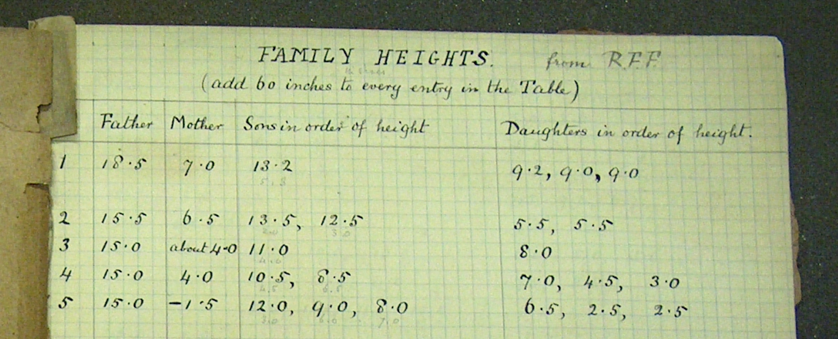
The idea of human assimilation of information is key. It isn’t information if a person can’t make sense of it. For instance, the height data shown in Figure 2.1 are recorded facts, measurements of the heights of adult children and their parents from the 1880s that today can easily be stored on a computer. Looking directly at those records is not a good way to reach conclusions about the relationships among the heights of mothers and fathers and their sons and daughters. To convince yourself of this, see what you can conclude by scrolling through the data available at http://tiny.cc/mosaic/galton.csv.
To create information from data requires transforming the data into a new form that can be digested by the human audience. There are many ways this can be done. Consider these statements which report patterns implicit in the long table of height data: “Husbands tend to be taller than their wives,” or “Taller parents tend to have offspring who are also relatively tall compared to the children of shorter parents,” or “parents’ height and children’s heights are positively correlated.”
The object of statistics and data science is to turn data into information. Narrowly seen, the role of data science is to support the collection and transformation of data so that statistics can do its work. There’s no hard boundary between data science and statistics; they both aim at the same target and their domains overlap considerably.
Statistics provides a language for constructing reliable data-driven statements comprehensible to a human. You’ve heard expressions in this language all your life. The point of this book is to help you learn the statistical language to use it effectively and to make sense of other people’s statistical statements.
Returning to the example of Figure 2.1, Francis Galton, who collected the height data also invented a way to summarize it: the correlation coefficient. You need to speak the statistical language a little bit to understand the summarizing statement, “heights of parents and their children are positively correlated.”
2.2 Tidy data in data frames
I’ve said that data is “anything that can be stored in a computer” and that the role of the statistician is to transform data into information. But how to carry out this transformation? “Anything stored in a computer” doesn’t provide much guidance about what techniques are most helpful for doing the statistician’s job.
In this section, you’ll meet a particular convention for organizing data that makes it much easier to apply the tools of stats. This convention is called tidy data. (Wickham 2014) In some ways, tidy data is common sense. But there is also some subtlety to the concept that rewards precise use of terminology and careful study and exact adoption of the conventions.
A simple but incomplete description of tidy data is organizing data into tables of rows and columns, the sort of thing spreadsheet software is sometimes used for. Table 2.1 is tidy data.
Table 2.1: The records from Figure 2.1 rewritten as tidy data.
| family | father | mother | sex | height | nkids |
|---|---|---|---|---|---|
| 1 | 78.5 | 67.0 | M | 73.2 | 4 |
| 1 | 78.5 | 67.0 | F | 69.2 | 4 |
| 1 | 78.5 | 67.0 | F | 69.0 | 4 |
| 1 | 78.5 | 67.0 | F | 69.0 | 4 |
| 2 | 75.5 | 66.5 | M | 73.5 | 4 |
| 2 | 75.5 | 66.5 | M | 72.5 | 4 |
| 2 | 75.5 | 66.5 | F | 65.5 | 4 |
| 2 | 75.5 | 66.5 | F | 65.5 | 4 |
| 3 | 75.0 | 64.0 | M | 71.0 | 2 |
| 3 | 75.0 | 64.0 | F | 68.0 | 2 |
| … and so on for 898 rows altogether. |
Table 2.1, like all tidy data, has a particular geometrical layout: rows and columns. We refer to such tables, containing tidy data, as a data frame.
The rows and columns of a data frame have different meanings.
- Each row is a unit of observation.
- Each column is a variable.
- Each cell – the intersection between a row and a column – is a value, that is, an observation or measurement.
2.3 Unit of observation
The unit of observation is the kind of thing each row corresponds to in the real world. For the data frame shown in Table 2.1, the unit of observation is an adult child. Galton recorded heights of 898 adult children in his notebook, so the tidy data frame has 898 rows.
In a properly arranged data frame, every row is about the same sort of observational unit. In Galton’s data, that unit is an adult child. Every value in the row for that child is an observation or measurement relating to that child: the child’s height, the child’s mother’s height, the sex of the child, the family unit to which the child belongs. Of course the mother and father are themselves people, and might have been included in the data frame. But we have no record of the height of the father’s mother, for instance.
Imagine a data frame about births. An obvious choice for the unit of observation is “a person being born.” Table @ref{tab:natality-intro} shows such a data table for the almost 4 million births in the US in 2014. For each baby (that is, “unit of observation”), the values of the variables sex, birth weight (in grams), mother’s age, and mother’s weight (in pounds) were recorded (as well as many others not shown here).
Table 2.2: Some of the 3,998,175 births recorded by the Centers for Disease Control in the US in 2014. The unit of observation is a birth.
| sex | b_weight | m_age | m_weight |
|---|---|---|---|
| F | 3629 | 23 | 211 |
| M | 2240 | 22 | 150 |
| M | 3750 | 24 | NA |
| F | 3657 | 40 | 293 |
| F | 3600 | 25 | 176 |
| F | 2126 | 27 | 200 |
| M | 3799 | 31 | 185 |
| M | 2065 | 27 | 129 |
| M | 2920 | 22 | 125 |
| M | 3330 | 30 | 170 |
| … and so on for 3,998,175 rows altogether. |
The layout of Table 2.2 is not the only way, of course, to organize data about births. For instance, if the interest is in the season-to-season variation in birth rate, Table 2.3 provides a suitable format. In Table 2.3 the unit of observation is a day in 2015. There are altogether 365 rows, one for each day in 2015.
Table 2.3: A births data frame in which the unit of observation is a day, not a baby. (Available as mosaicData::Births2015.)
| date | births | wday |
|---|---|---|
| 2015-01-01 | 8068 | Thu |
| 2015-01-02 | 10850 | Fri |
| 2015-01-03 | 8328 | Sat |
| 2015-01-04 | 7065 | Sun |
| 2015-01-05 | 11892 | Mon |
| 2015-01-06 | 12425 | Tue |
| 2015-01-07 | 12141 | Wed |
| 2015-01-08 | 12094 | Thu |
| 2015-01-09 | 11868 | Fri |
| 2015-01-10 | 8014 | Sat |
| … and so on for 365 rows altogether. |
Exactly the same births in Table 2.3 can be presented in the form of Table 2.4 where the unit of observation is a day of the week in 2015 and the recorded number of births is the sum for that day over the whole year.
Table 2.4: Birth data with day-of-the-week being the unit of observation.
| wday | births |
|---|---|
| Sun | 384686 |
| Mon | 610448 |
| Tue | 654462 |
| Wed | 638513 |
| Thu | 640422 |
| Fri | 615397 |
| Sat | 434569 |
The simple re-arrangement of data from Table 2.3 to Table 2.4 helps to convey information: it’s easy to see that Saturdays and Sundays have lower numbers of births than the other days in the week.
Each of the data frames 2.2 and 2.3 and 2.4 reflects the same facts – the number of births in the US in 2015 – they simply have a different unit of observation. Looking at the facts in different ways can give us new information.
It’s easy to imagine how one might go about transforming a data frame like Table 2.2 where the unit of observation is a birth into another data frame recording the same facts but where the unit of observation is a day of the year or a day of the week. Words used to describe the operation include data “reduction,” “aggregation,” “summation,” and “tabulation.” Such aggregations are one of the basic operations of data wrangling.
On the other hand, given aggregated data, it’s impossible to disaggregate them without going to the original source – the raw data – on which the aggregation was performed. Keep in mind that “raw data” is simply data. Usually it is in a form too cumbersome to be assimilated by the human reader. The data scientist and statistician refine raw data into a form that’s easily assimilated: information.
Historically, little distinction was made between the presentations of data intended to guide human reasoning and the formats used for archiving purposes: both were printed tables, whether on paper or computer punch cards. Printing was possible only if the raw data were reduced in size to something that fits in the pages of a book or a stack of computer cards. Consequently, people became used to thinking about data as aggregated tables. Since each form of aggregation produces a data table suitable for some purposes but not others, the available data often could not be used to address new questions. Today, vast quantities of raw data can be stored and accessed on computers and, importantly, aggregations can be speedily and easily performed by software. So it’s best to store data with as fine a unit of observation as possible, e.g. individual births instead of tallies over days or weeks or states or sexes, ….
2.4 Variables
Each column of a data frame is a variable.4 The word “variable” reflects the values varying from row-to-row. Note that “variable” has different meanings in different contexts. In everyday life, variable means “changing” or “able to be changed.” In algebra, a variable is an unknown quantity, typically written x. When it comes to tidy data, variables are known and recorded. The individual entries in a column are values of that column’s variable.
It’s important to distinguish between two main types of values:
- *****Quantitative*****: a number.
- *****Categorical*****: a label, typically written using characters.
In Table 2.2 the baby_weight variable is quantitative, while sex is categorical.
In tidy data, the value of any particular variable is the same kind of thing for every observational unit. For instance, the baby_weight variable is a number giving the weight of the newborn baby in grams. It wouldn’t be tidy data if there was some other kind of thing recorded as a value for babyweight like “big” or “tiny”. Similarly, the categorical variable sex has values that are always the labels “F” or “M”. It wouldn’t be tidy data if an entirely different kind of thing, say, “Golfer”, were recorded under sex.
For a categorical variable, the set of possible values of a variable are called the levels of the variable. In the individual-birth sex variable, the set consists of "F" and "M". For a quantitative variable, the each value is, naturally, numbers.
Quantitative variables typically represent some real-world a count or a quantity with units, e.g., inches, years, millimeters of mercury (mmHg). In tidy data, the units of the quantitative variable are not part of the value; they are implicit. A good reason for this is that, as required for tidyness, the a variable’s unit must be the same in every row. This is part of what it means that all the values are the same kind of thing.
2.5 Example: Categories of smoking
In the 1950s, smoking was much more prevalent (in the US) than today. But by the early 1960s, evidence for the harmful effects of smoking was becoming hard to ignore. Perhaps most famously, the US Surgeon General5 The Surgeon General is the head of the US Public Health Service and the most senior official spokesperson about public health in the US. issued a report in 1964 establishing a causal link between cigarette smoking and lung cancer, the precursor to many successful public health initiatives limiting advertising, raising taxes on cigarettes, and banning smoking indoors or in public places.
Smoking during pregnancy was another matter of concern. One of the first studies of this covered 13,083 pregnancies in Oakland, CA from 1960 to 1967. (Yerushalmy 1971) Some of the data from the study, covering 1236 pregnancies in 1961-1962, have been preserved (Speed and D 2000) and is available as the mosaicData::Gestation data frame.
The Gestation data frame includes three categorical variables about the mother’s smoking:
smoke, which answers the question: Does the mother smoke? The levels forsmokeare never, still smokes, until current pregnancy, once did, not now.time, giving the time since quitting smoking. The levels are never smoked, still smokes, within 1 year, 1 to 2 years ago, 3 to 4 years ago, 5 to 9 years ago, 10+ years ago.number, the number of cigarettes smoked per day. Actually,numberis not recorded as a quantitative variable. Instead, the was collected as a range of numbers in the form of categories: never, 1-4 cigarettes, 5-9 cigarettes, and so on up to 60+ cigarettes.
2.6 Metadata
Data frames should always come with metadata: data about the data. Metadata should include a description of what each variable represents. A proper description of a categorical variable should explain each allowed level, that is, what is the meaning of each of the set of possible values. For quantitative variables, the units of the value should be recorded. For instance, baby_weight is in grams, while mother’s weight before pregnancy is in pounds.
Many spreadsheet users place notes in the sheet to document what’s what. This common-sense practice can, in fact, trip you up. Metadata should be recorded apart from the data itself, say in a separate document. The metadata is intended for human eyes, whereas a data frame is intended for computer digestion. Separating the two makes it easier to use software.
Often the document containing meta-data is called a codebook. This colorful term is not about secrecy but the now-obsolete practice in early computer programs to store categorical data as simple integers. For instance, a variable sex might have had levels 0 or 1. Which number is for which sex? That’s what the codebook was for.
2.7 Example: Business in Babylon
Figure 2.2 shows an example of Babylonian cuneiform, where data were recorded as stylus marks on clay tablets.

Figure 2.2: A cuneiform tablet inscribed with a receipt for a tax transaction. (ca. 1634 BC)
The data recorded in the cuneiform writing and seals was presumably important for the person paying the tax. Data in the form of the image itself is useful for those who can read cuneiform studying daily life 3500 years ago. Still more data, data about the tablet image data, allowed me to locate it on the internet. Such data about data is often called metadata. Table 2.5 is an excerpt from the metadata for the tablet image:
Table 2.5: Metadata describing the Babylonian cuneiform tablet.
| field | value |
|---|---|
| Date | -1634 - -1634 ca. 1634 B.C. |
| Extent | 4 x 3.8 x 2.3 cm (1 5/8 x 1 1/2 x 7/8 in.) |
| Medium | Clay |
| Provenance | Purchase, 1886 |
| Source | 86.11.104 |
| Spatial | Mesopotamia probably from Sippar |
| Agg Provider | Metropolitan Museum of Art |
| URL root | http://www.metmuseum.org |
| Shown At | /art/collection/search/321701 |
2.8 Other data forms
Data comes in many forms that do not have identified rows and columns, units of observation and variables. Figure 2.3 shows a photographic record of a tipi ring, the remnants of encampments of original residents of the American west.

Figure 2.3: A photograph of a tipi ring. (source: Linda Hanney)
However tidy the ring in Figure 2.3, and even though the photo is data (it can be stored on a computer), the photo is not tidy data. After all, for tidy data there is always rows and columns, a unit of observation and variables.
Often, one of the first steps in working with such records is to translate them into tidy data. For instance, for tipi rings the unit of observation might be an individual ring and the variables shape, enclosed area, material, latitude and longitude, direction in which the opening faces, and so on.
As another example, Figure 2.4 shows a recording of local shaking of the Earth’s surface during an earthquake.
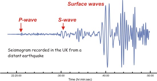
Figure 2.4: A seismogram recorded during an earthquake. Annotations show the arrival of two kinds of waves.
In studying earthquakes, seismologists extract from such recordings features of the recording themselves, which can be placed in a tidy-data format. For instance, an individual seismogram might be one row in a data frame with variables giving the p-wave arrival time, the s-wave arrival time, and an identifier for the earthquake. There are usually many seismographs at different locations recorded for each major earthquake, so the unit of analysis would be a seismogram, not an earthquake.
In studying earthquakes, seismographs from different locations are processed to find the latitude, longitude, and depth of the earthquake, as well as the magnitude, and other “source parameters” such as the “slip azimuth.” A data frame with this information would have a different unit of observation: not a seismogram but an earthquake.
Transforming recorded data into tidy data is often an important step in studying a phenomenon, be it the historical life patterns of Native Americans or the forces that shake the earth.
2.9 Response and explanatory variables
Variables in tidy data have individual names, e.g. age, temperature, energy_use. As mentioned in Chapter 1 there are also generic names that reflect how variables are presented or used in constructing a statistical summary:
- Response variable
- Explanatory variables
- Covariates
These labels are not intrinsic to the data itself, but arise from the uses to which we put data. For instance, suppose you want to make a prediction of how much energy a house will use in the upcoming month. You have data on the electric and natural gas energy use in previous months, together with average outdoor and indoor temperature in those months, the number of occupants in the house, and so on. To predict the amount of natural gas used, you will be a model with natural gas usage as the response variable. This is just a way of saying that the output of the prediction model will be natural gas usage. To inform the prediction, you might use outdoor and indoor temperature. These will be the explanatory variables in the model. The word covariate describes an explanatory variable in which you, the modeler, have no direct interest but which you recognize should be included in the model to give a faithful representation of how the system works.
You’ll see the labels response variable and explanatory variables used in the next chapter as we make statistical graphics. By convention, the response variable will be displayed by the vertical axis and explanatory variables displayed by the horizontal axis, color, and “faceting” of the graph.
2.10 Exercises
Problem 1: The US Department of Transportation has a program called the Fatality Analysis Reporting System. FARS has a web site which publishes data. Figure 2.5 comes from their web page.
Figure 2.5: National statistics from the US on fatalities from motor-vehicle accidents.
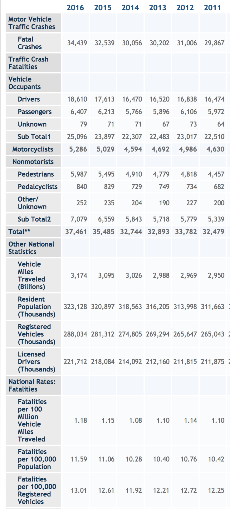
For several reasons, the FARS table is not in tidy form.
Some of the rows serve as headers for the next several rows, but don’t contain any data. Identify those headers.
- In tidy data, all the entries in a column should describe the same kind of quantity. You can see that all of the columns contain numbers. But the numbers are not all the same kind of quantity. Referring to the 2016 column:
- What kind of thing is the number 34,439?
- What kind of thing is 18,610?
- What kind of thing is 1.18?
In tidy data, there is a definite unit of observation that is the same kind of thing for every row. Give an example of two rows that are not the same kind of thing.
Identify a few rows that are summaries of other rows. Such summaries are not themselves a unit of observation.
Problem 2: A commonly used indicator of population health is “life expectancy at birth.” Globally, the 2016 estimate of life expectancy at birth is 72.0 years (74.2 years for females and 69.8 years for males). Many people mis-interpret this to mean that they are most likely to live to to that age. Instead of looking at life expectancy at birth, a person interested in his or her own prognosis should look at life expectancy at their current age. For instance, in 2016 life expectancy at birth was 71.9 years (77.2 for females, 65.7 for males). But at age 60, life expectancy is 19.4 more years (21.8 for females, 16.1 for males). [Source: World Health Organization]
Many countries publish detailed tables about life expectancy at each year of age. For the United Kingdom, a spreadsheet file containing this data is available here (with a cached version here). We’ll use the data in this file in later chapters. For now, let’s focus on the format of the file itself.
- There are several tabs in the spreadsheet file. Which ones include metadata of the sort that should be in a codebook file?
- What is the unit of observation?
- How would you reformat the table so that sex is a variable rather than a heading?
- If you were to put the data for both sexes split up among all the year tabs (e.g. 2016-2018, 2015-2017, 2014-2016) into one big tidy table, how would you modify the format from your answer to (5)?
Problem 3: The following table is a small excerpt from a table published by the US Environmental Protection Agency (EPA) about the fuel consumption of motor vehicles sold in the US. (See documentation for SDSdata::MPG.)
The name 2Dr Pass Vol stands for “2 door vehicle passenger volume” (in cubic-feet). Similarly the variables with Lugg refer to luggage volume.
| Mfr Name | Carline | 2Dr Pass Vol | 4Dr Pass Vol | Htchbk Pass Vol | 2Dr Lugg Vol | 4Dr Lugg Vol | Htchbk Lugg Vol |
|---|---|---|---|---|---|---|---|
| Mitsubishi Motors Co | MIRAGE | NA | 86 | 86 | NA | 17 | 17 |
| aston martin | DB11 V12 | 72 | NA | NA | 9 | NA | NA |
| BMW | COOPER CONVERTIBLE | 76 | NA | NA | 5 | NA | NA |
| FCA US LLC | Giulia | NA | 100 | NA | NA | 12 | NA |
| Ferrari | Portofino | 75 | NA | NA | 5 | NA | NA |
| Ford Motor Company | FORD GT | 43 | NA | NA | 0 | NA | NA |
| General Motors | CASCADA | 82 | NA | NA | 9 | NA | NA |
| Honda | ILX | NA | 89 | NA | NA | 12 | NA |
| … and so on for 21 rows altogether. |
Each of the “Vol” columns mixes together two features of the vehicle: the volume and whether the car is or is not a 2-door, a 4-door, or a hatchback.
- Why are so many of the “Vol” columns marked
NA? - The first row displayed has some redundant entries. Why?
- Re-organize the data frame so that it has a variable that is exclusively about volume, another that is exclusively about 2- versus 4-doors, and another exclusively about whether the car is a hatchback. As you do this, keep in mind that the names of the variables in the original are long-winded, include spaces, and often start with a number. These are inconvenient features for a variable name being handled by software. Try to use variable names that will be convenient for a data scientist working with the data.
Problem 4: Glaucoma is a disease of the eye that is a leading cause of blindness worldwide. For those people with access to good eye health care, a diagnosis of glaucoma leads to treatment as well as monitoring of the possible progression of the disease. There are many forms of monitoring. One of them, the visual field examination, involves making measurements of light sensitivity at 54 locations arrayed across the retina. The data frame shown below (provided by the womblR R package) records the light sensitivity for one patient at each of the locations. Data from two visits – an initial visit marked 1 and a follow-up visit marked 2 which occurred 126 days after the initial visit – are contained in the data frame.
| location | day | visit | sensitivity |
|---|---|---|---|
| 1 | 0 | 1 | 25 |
| 1 | 126 | 2 | 23 |
| 2 | 0 | 1 | 25 |
| 2 | 126 | 2 | 23 |
| 3 | 0 | 1 | 24 |
| 3 | 126 | 2 | 24 |
| 4 | 0 | 1 | 25 |
| 4 | 126 | 2 | 24 |
| 5 | 0 | 1 | 26 |
| 5 | 126 | 2 | 17 |
| … and so on for 108 rows altogether. |
- What is the unit of observation?
- Suppose a third visit was made and the new data were included in the table.
- How many columns would the revised table include?
- How many rows would the revised table include?
Note that
dayandvisithave a very simple relationship. Construct a separate table that has all the information relatingdaytovisit. The unit of observation should be “a visit”.Each
locationis a fixed point on the eye’s retina that can be identified by (x, y) coordinates. Here is a map showing the position of each location.
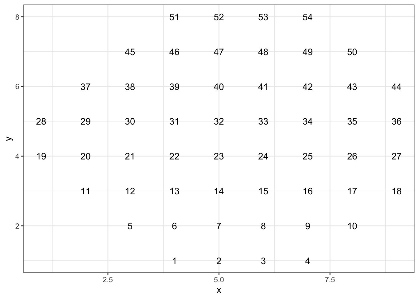
Notice that location 1 has position (4, 1) and location 2 has position (5, 1). Imagine a data frame that records the position of each location.
- How many columns would the data frame have and what would be sensible names for them?
- How many rows would the data frame have?
- Write down the data table for positions 1, 2, 3, 4, 5, and 6.
Problem 5 List what’s not tidy about this table.

Problem 6 The data table below records activity at a neighborhood car repair shop.
| mechanic | product | price | date |
|---|---|---|---|
| Anne | starter | 170 | 2019-01-12 |
| Beatrice | shock absorber | 78.42 | 2019-01-12 |
| Anne | alternator | 385.95 | 2019-01-12 |
| Clarisse | brake shoe | 39.5 | 2019-01-12 |
| Clarisse | brake shoe | 39.5 | 2019-01-12 |
| Beatrice | radiator hose | 17.9 | 2019-02-12 |
| … and so on for 456 rows altogether. |
The codebook for a data table should describe what is the unit of observation. For the purpose of this exercise, your job is to comment on each of the following possibilities and say why or why not it is plausible as the unit of observation.
- a day.
- a mechanic.
- a car part used in a repair.
Problem 7 The data about motor-vehicle related fatalities shown in Figure ?? are not tidy. Table 2.6 is a re-organized version of the data.
Table 2.6: Tidied data on motor-vehicle fatalities.
| year | crashes | drivers | passengers | unknown | miles | resident_pop |
|---|---|---|---|---|---|---|
| 2016 | 34439 | 18610 | 6407 | 79 | 3174 | 323128 |
| 2015 | 32539 | 17666 | 6213 | 71 | 3095 | 320897 |
| 2014 | 30056 | 16470 | 5766 | 71 | 3026 | 318563 |
| … and so on for 25 rows altogether. |
- In Table 2.6, what is the unit of observation?
- Is Table 2.6 tidy data?
- For the purpose of this exercise, one of the numbers in Table 1 was been copied with a small error in Table 2.6. To see which it is, you’ll have to refer to the original table. Find that number and tell:
- The quantity presented in the variable
milesis not actually in miles. It has other units. Referring to Figure ?? …- What are the actual units?
- Where should the information in (a) be documented?
Problem 8 The meta-data for Table ?? should include a description of each variable, its units, and what it stands for. Write such a description for the variables crashes and resident_pop. You can refer to Figure ?? for information.
References
Speed, T, and Nolan D. 2000. Stat Labs: Mathematical Statistics Through Applications. New York: Springer. https://www.stat.berkeley.edu/users/statlabs/labs.html#babies.
Wickham, Hadley. 2014. “Tidy Data.” Journal of Statistical Software 59 (10). https://www.jstatsoft.org/article/view/v059i10/.
Yerushalmy, J. 1971. “The Relationship of Parents’ Cigarette Smoking to Outcome of Pregnancy—Implications as to the Problem of Inferring Causation from Observed Associations.” American Journal of Epidemiology, 443–56. https://doi.org/10.1093/oxfordjournals.aje.a121278.