Chapter 18 Cross validation
THESE ARE NOTES for an early draft.
Talk about systems where cross-validation is part of the model-building method. Then we talk about training/validation/test set
The connect-the-dots model always has a good in-sample prediction error. How does it do out of sample?
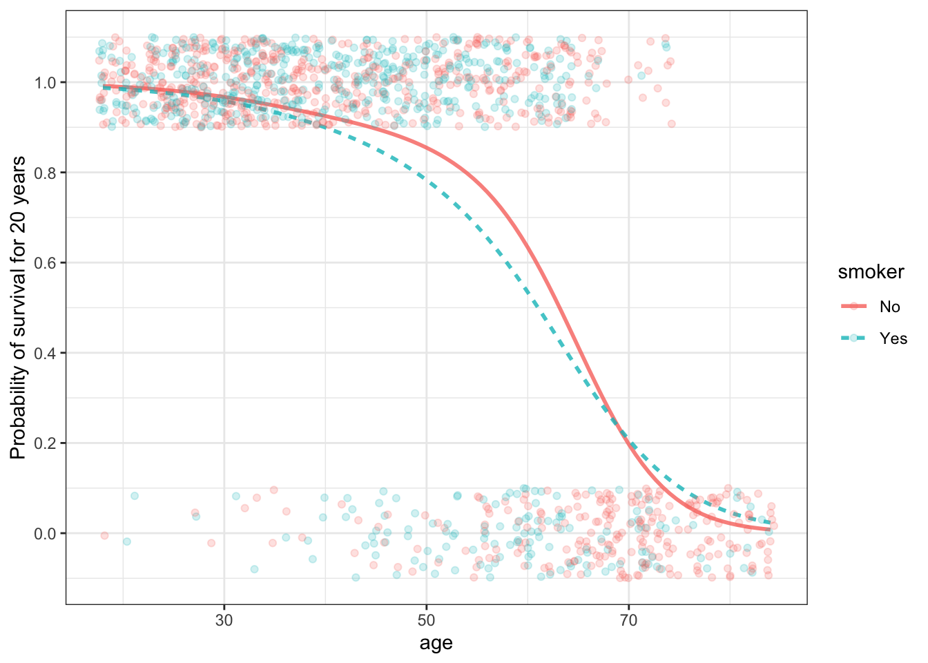
Build a tree model with many more splits. Is it better at predicting in-sample? Out-of-sample? Refer to the dip in survival for the people in their 50s as a likely example of overfitting.
Exercise: Do the smoking again using a very high-order natural spline. Does it actually help prediction.
18.1 Example: Cooling water (again)
Let’s return to the models we built of the temperature of water as it cools to room temperature. In Table 16.4 we calculated the room mean prediction error of four models. However, that table was based on using the training data, rather than testing data, to evaluate the model performance. Figure 18.1 shows the results from cross-validation.
For the very simplest model function, a single exponential, the cross-validated error is somewhat higher than the error found from the training data: about 2.1 degrees compared to the 1.5 in Table 16.4. For the two-exponential model, the cross-validated error is also somewhat higher. Comparing the cross-validated errors from the one- and two-exponential models indicates that the two-exponential model is genuinely better than the one-exponential model, consistent with the water being in contact with two media: the cup and the room air.
Figure 18.1: Cross-validation applied to the cooling-water models in Figure 16.5.
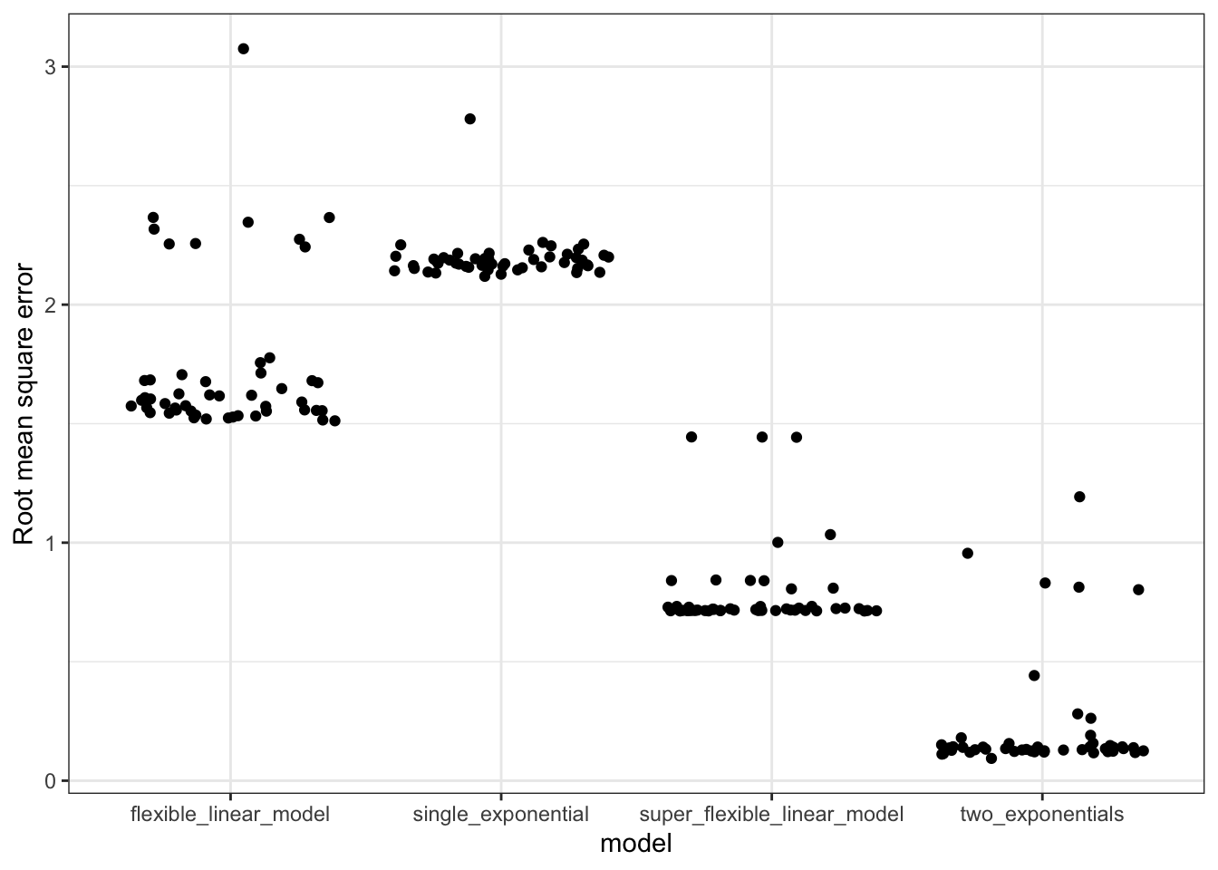
For the flexible and super flexible linear models, the cross validated error is much higher than the error calculated from the training data. Using the training data, the super flexible model had a much smaller error than the two-exponential model. But with cross-validation, it’s evident that the opposite is true: the two-exponential model beats out all the other models.
18.2 Training and testing data
Recall the model-building process as it has been introduced so far:
- You have some data, including a response variable and explanatory variables of interest (including covariates, if any).
- You choose a family of functions to represent the relationship between the response and explanatory variables (taking into account the covariates).
- The computer uses the data to find a particular member of the selected family of functions that best matches the patterns in the data. This is called training or fitting the model.
We haven’t discussed in any detail the means by which the computer solves the problem in (3). This is the subject of Chapter @ref(model_training), but for now it will be helpful to outline how model training works.
Each function family comes with a quantitative measure of fit: how well any potential candidate from the selected family of functions matches the data. The computer starts with a guess. and then makes proposes a small modifications to the function. (The mechanisms for making such proposals can be extremely interesting in their own right, but those mechanisms are not our concern here.) While doing this, the computer keeps track of the measure of fit. If the proposed modification results in a better fit, that modification is accepted, replacing the previous best guess. If the proposed modification results in a worse fit, the modification is not accepted and the computer creates a new proposal for a modification. The process continues refining the model in this way until it can no longer readily find improvements. That last function becomes a kind of king of the hill: a function whose fit is better than all those that can be generated from it by the proposal mechanism.
This brings us to a fourth phase in the model building process:
- Evaluating the computer-generated model in terms of how well it achieves your own goals for the model. For example, a model used for medical diagnosis certainly should get the diagnosis right as often as possible, but it should also avoid mis-diagnoses that are particularly harmful to the health of the patient.
It’s tempting to hope that the automatic training process would always generate the best function for your purpose in modeling. But your purpose may not align well with the function family’s quantitative measure of fit, for instance by not incorporating information about the differences in harm to the patient caused by the various possible mis-diagnoses.
Another reason not to accept at face value the model generated by the automatic training process is that the model training process tends to overstate how well the fitted model performs. The basic problem is that the training process can lock in on idiosyncracies of the training data. For this reason, it’s best to use different data to evaluate the model in step (4) than was used in step (3) to train the model. This new data is often called testing data. Sometimes the testing data is genuinely new data, coming from a different source or collected at a different time than the training data. Other times, the testing data was available for use in training in step (3), but you intentionally withhold it from the training process in order to have valid testing data.
18.3 Training, tuning, and testing data
From this book …
Segmenting your data into training, tuning and testing sets. Consider the brief discussion on selecting a tuning parameter for LASSO and Ridge regression in the previous chapter. The tuning set can be used to select that parameter, then the final model can be validated with the testing set.
Repeating k-fold CV multiple times. Performing k-fold CV one time is not too different than the single training and testing set approach, data is segmented randomly into sets. A different random permutation will result in a different RMSE (we saw this above!). It is possible to repeat the k-fold CV multiple times and aggregate all the results. If computational power allows, this is typically done in practice.
18.4 POSSIBLE EXAMPLE
It’s possible to add increased flexibility to logistic models, as well as interactions between explanatory variables.
Figure 18.2: (ref:w-logistic-cap)
When is the added detail meaningful: confidence bands
Figure 18.3: (ref:w-svm-cap)
18.5 ANOTHER POSSIBLE EXAMPLE
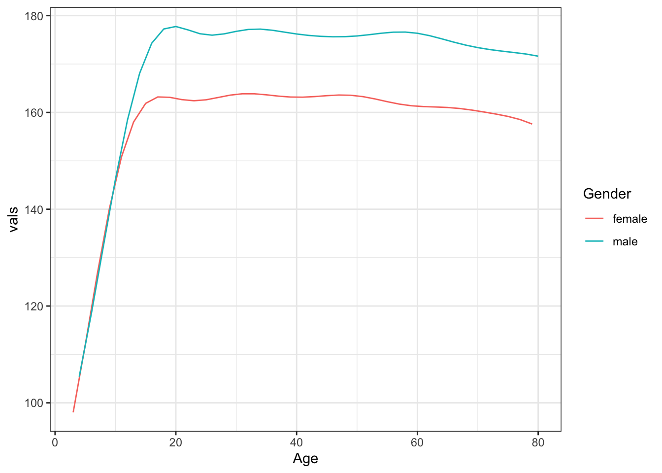
18.6 Example: Tree regression
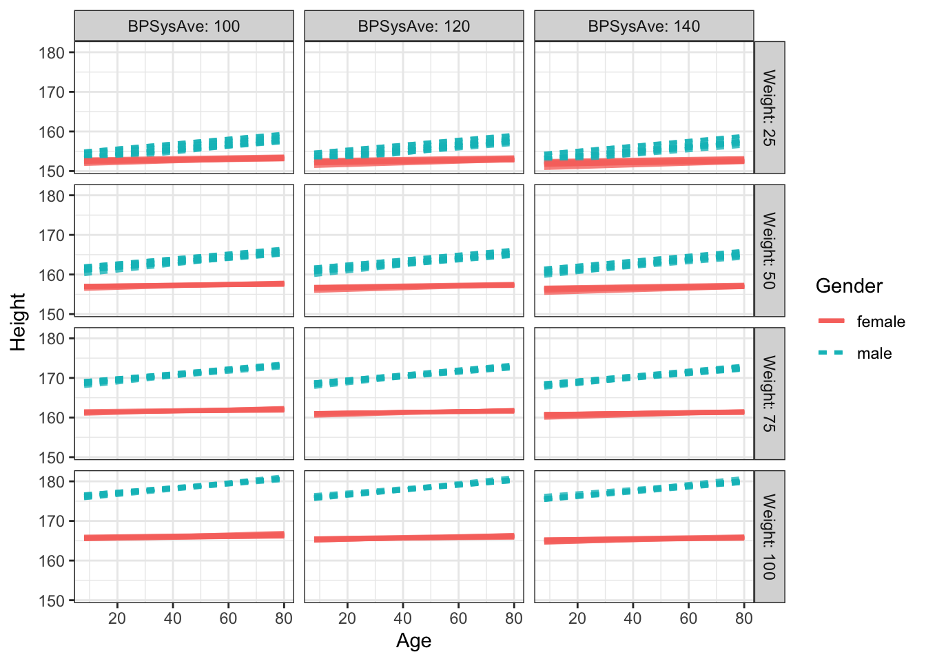
An example of a tree regression model: Height versus age, sex, weight, blood pressure, …
It should have an interaction.
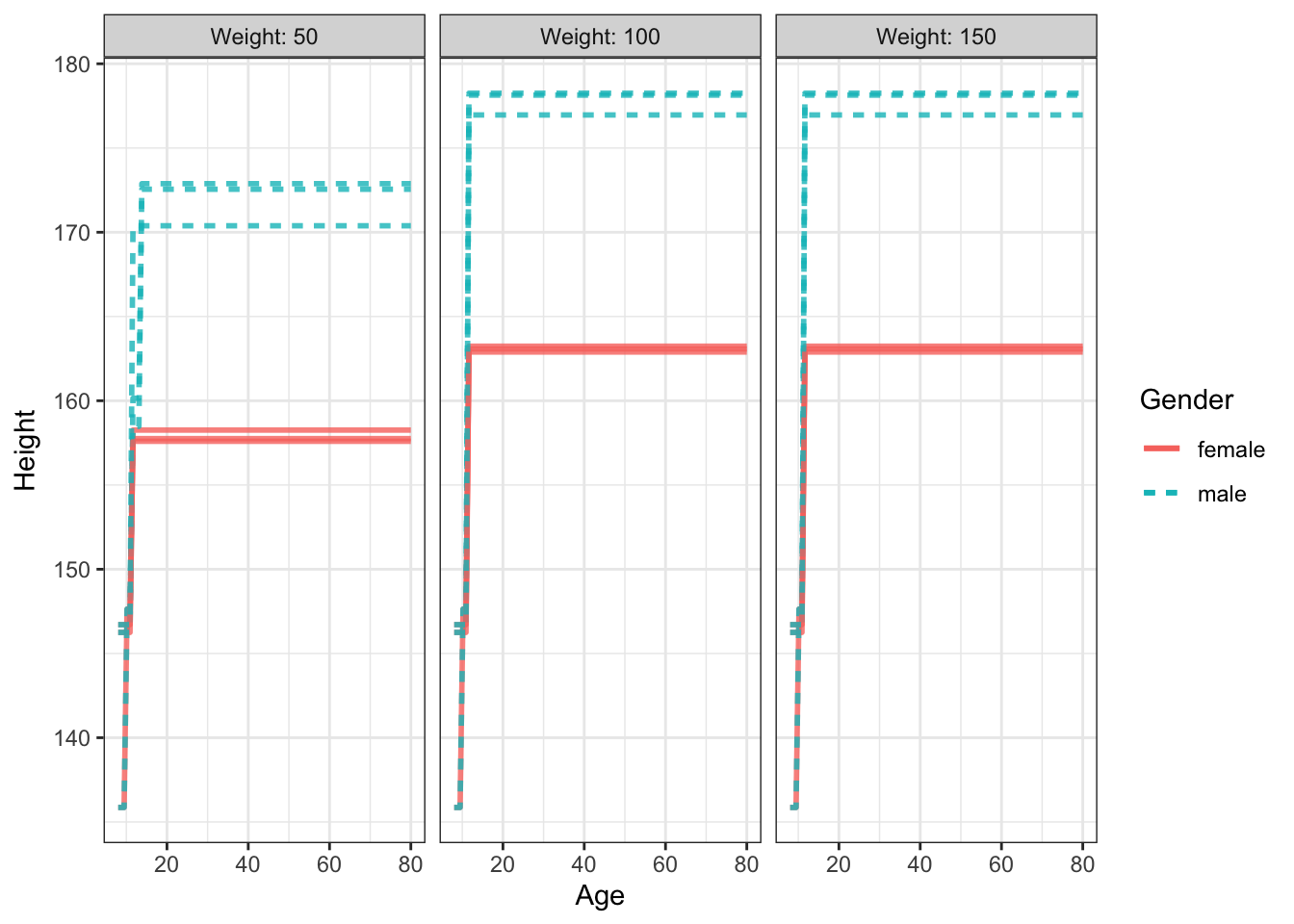
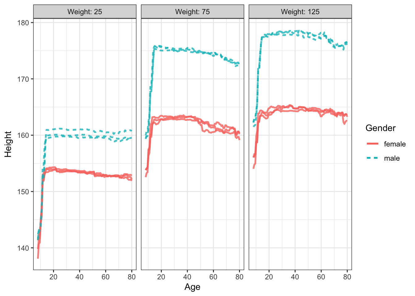
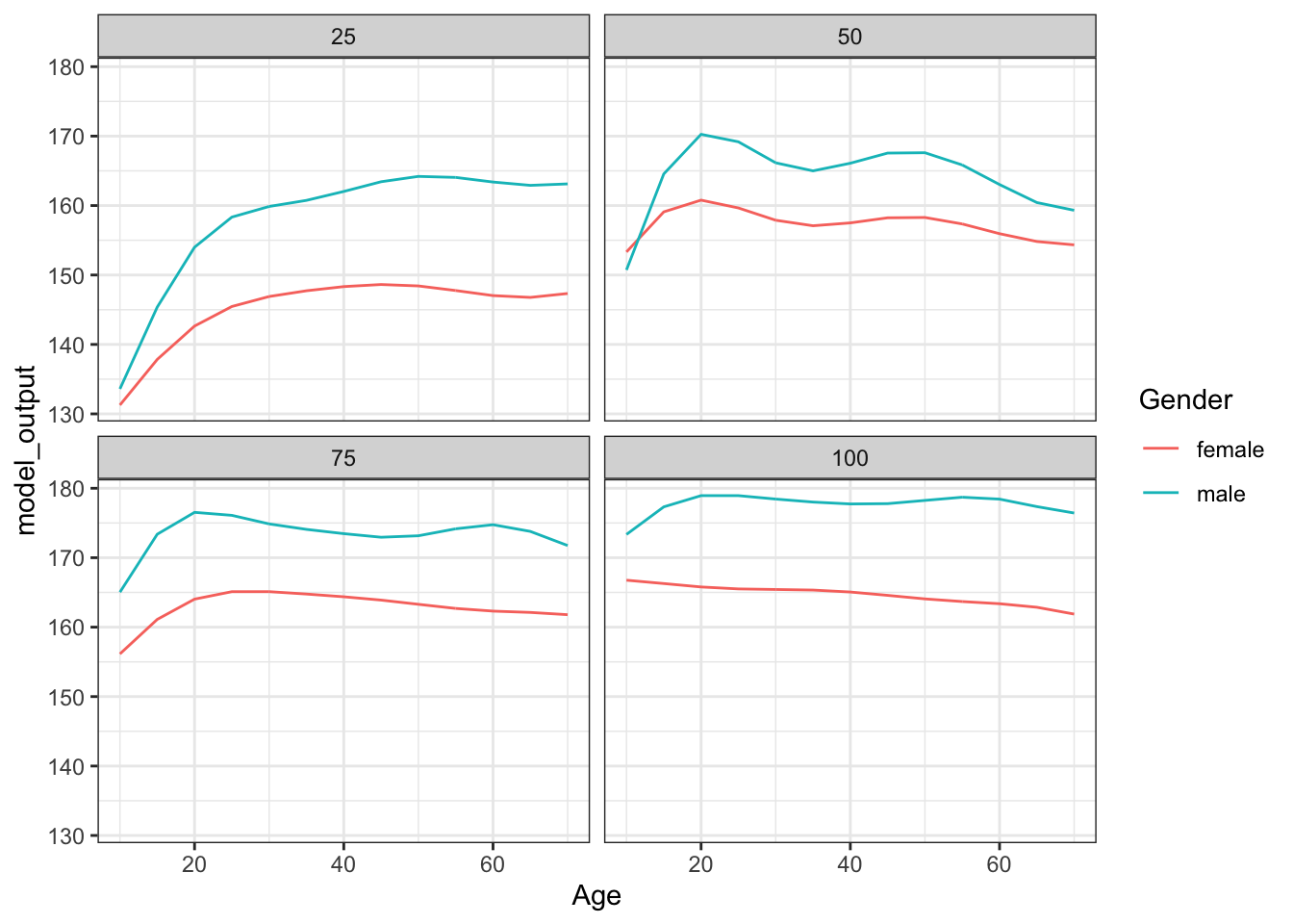
SVM is too smooth in this case: do we really want to treat childhood and adulthood the same in terms of height? So, stratify them.
… Discovering explanatory variables …
Showing the ability to find the relationships … rpart, randomForest
Hmod_lm_2 nails it down (in ANOVA) to mainly Weight and BMI. That’s right, but not really what we were looking for!