Chapter 8 Case study: from purpose to result
The previous chapter outlined an abstract set of steps for the data-related part of a research project. This chapter illustrates some of those steps using a simple setting. As you read, keep in mind that there is more to data science than data. Focusing solely on the modeling of data without considering the other steps can easily lead you astray.
I. Know your purpose
The question to be answered addressed in this example might at first come across as simple:
For people who drive long distances on the highway, how fast should you drive?
Your client is the person or organization who is to be informed and guided by your work. Let’s imagine for now, that the client is a group of friends or fellow students. Knowing who your client is helps you determine
- The resources available to support your work.
- The overall setting in which the results of your work will be used.
- The broader objectives that are important to your client. For instance, the several objectives to be informed by your work are:
- Don’t spend too much on gas.
- Avoid long hours of driving because 1) you have better things to do and 2) driving while bored and tired is dangerous.
- Be safe.
- Avoid speeding tickets.
- How best to communicate your results, including being understood, being credible, and being genuinely useful.
II. What information you have or need to gather
At the onset of any modeling project, it’s a good idea to study what’s already known about the sort of system you’ll be studying. An internet search can be a good start, keeping in mind that much information on the internet is not reliable. If you don’t yet know much about the system under study, it may be hard to know what’s reliable and what not. At first, you may need to base judgment on superficial signs of reliability: precise use of vocabulary, citation of sources, publication in professional journals, and so on.
There may be people in your organization who have experience with the system, even if they don’t have technical skills working with data. Interview them to find out how they think about the problem at hand. (But first do a bit of reading so you can ask reasonable questions.) Take what experts have to say seriously. This is especially important when your project is similar to others that have been successfully completed. But there are also times when expert opinion is misleading or wrong or when what’s needed is fresh insight. You’ll need to use judgment to decide how much weight to give expert opinion.
Looking at the objectives you uncovered in Step I, you’ll want to know …
- How does driving speed affect fuel use?
- What are the “better things you have to do” and what value do they really have?
- How is safety affected by driving speed?
- What are the legal constraints?
An internet search on how speed affects fuel economy quickly turns up many blog posts and question-and-answer forums. These seem mostly to be empty and unsubstantiated reiterations of conventional wisdom. But there are exceptions. Some point out that internal combustion engines usually have an optimal operating speed that depends on the engine design. Others distinguish between “fuel economy” (in miles per gallon) and “fuel consumption” (in gallons per 100 miles or liters per 100 km).
A web site oriented to professional long-distance truckers claims that an “average” truck gets 5.9 miles per gallon (of diesel fuel) and that a 10 mile-per-hour increase in speed reduces that to 4.5 miles per gallon. Whether this is relevant to the kind of car you drive is questionable, but it does give you a rough idea that going 10 miles per hour faster reduces fuel economy by 25%. This might be applicable to your car. Judgment is needed. When you find such statements, make note of them recording as well the source so you can document what you are finding.
A 1981 article in the research journal Energy reports on 350 car models from 1965 to 1977. (Greene 1981) It reports:
Average decreases in fuel economy for all cars in the sample were 8% from 64 to 80 km/hr, 12% from 80 to 97 km/hr, and 13% from 97 to 113 km/hr. Sensitivity of the fuel consumption rates to speed increased with increasing speed and decreasing engine size. [Note: This translates to a roughly 10% decrease in fuel economy for a 10 mile-per-hour increase in speed.]
This sounds authoritative, but even if it is, cars have changed a lot from 1977. Judgment.
A 2018 briefing, “Modeling the relationship between vehicle speed and fuel consumption,” given to the Transportation Research Board of the National Academies of Science, Engineering, and Medicine, provides an impressively detailed account. It incorporates not just vehicle speed, but road grade (slope), road curvature, and roughness of the pavement. The report covers vehicle types from small hatchbacks to tour busses and large trucks. There’s consideration of different road and intersection types, for instance, traffic lights versus traffic circles (roundabouts).
Will you need to include all this detail in your model? Judgment is called for. Keep in mind the purpose of your work: to find the best driving speed for your vehicle in interstate highway driving. The purpose of the models described in the briefing was very different, to guide policy formation about speed limits and road design.
We’ll suppose that you judge that you’ll need to collect some data that’s relevant to the cars used by your client.
The other things you have to do is really a question of how much your client value its time. One way to address this is to look at people’s forgone dollar earnings. For your friends or your fellow students a reasonable placeholder amount might be $10 per person-hour. Another placeholder is needed for the number of people in the car. Let’s set this to 2.
The reason to call these two numbers placeholders is that you or your client might decide to change them. Whatever form your results take, it should be obvious to the client how to modify the conclusions if the numbers were different.
“Safety first,” as the expression goes. In reality, we balance safety sensibly against other priorities. For instance, if safety were the only objective, we wouldn’t be driving. It’s very hard to come up with a meaningful “value of safety” as we did, for instance, with the value of “the other things you have to do.” Usually, we start with a baseline like, “Highway driving is a reasonably safe thing to do,” and then check that our actions don’t impose a dramatic decrease in safety.
One study about driving speed and safety reports that the risk of a fatal accident more-or-less doubles with an increase of 10 mph at highway speed. The overall accident rate increases by about 50 percent. But this study involves all kinds of driving. Interstate highway driving is much safer than other sorts of driving. Auto accidents are much more common at night. And almost half of night-time accidents are associated with alcohol. Road conditions due to weather are an important factor in safety in many regions. Fatique is another important cause of accidents. Shorter driving times (that is, higher speeds) provide less opportunity for fatique. Experience suggests that safety is enhanced by driving at a similar speed to other vehicles on the road. A reasonable overall judgment is that for the kind of driving we’re modeling and for reasonable driving speeds, safety is not a decisive issue. But notice how much detail we had to know about safety – road type, fatique, avoidable conditions like weather and alcohol – to make this judgment.
The legal constraints on driving speed are a somewhat complex issue. One perspective is that the posted speed limit sets the upper constraint. On a highway, the lower limit is often something like 40 miles-per-hour (mph). But the posted speed limit varies widely from one place to another. In some places 50 mph, in others 85 mph. In reality, many people drive somewhat faster than the posted limit. This suggests that, to be useful, our report should consider a wide range of possible driving speeds, say up to 85 mph.
A very important but often neglected question to ask is how precise the results of your work will need to be. Would it matter if your estimate of the extra fuel consumed by faster driving were off by 10%, 25%, or even 50%? You may not be able to answer this question at first, but until you have more insight, targeting a precision of about 25% is reasonable. This may go against your intuition, shaped in part by your mathematics education which emphasized exact answers to toy problems. Two statistical epigrams to keep always in mind are these:
Far better an approximate answer to the right question, which is often vague, than an exact answer to the wrong question, which can always be made precise. – John Tukey (1915-2000)
All models are wrong, but some are useful. – George Box (1919-2013)
Or, from a more literary perspective,
The best is the enemy of the good. – Voltaire (1694–1778)
Often, moving forward on a problem requires approximation and imprecision. Don’t chase after unreachable perfection, but do take care to report the imprecision of your results along with an estimate of what the influence might be of factors you didn’t include in your models. A valid outcome of a data science project is to give an answer based on the available knowledge and data and to point out how additional data might improve the answer.
The above review of what we already know is helpful in several ways. We’ve concluded that common sense and not statistical guidelines handles the issue of safety. We found out that we don’t know much about fuel economy and vehicle speed, and that what’s published may not be reliable or relevant. This suggests looking into collecting relevant data. We’ve also decided that the wide range of legal speed limits means that our investigation needs to take a broad point of view. And, tentatively, we’ll make do with the assumption that the value of time saved will be about $20/hour, though we might change this later.
III. Design a data collection plan
First, is it even possible to collect relevant data? Suppose you have access to a vehicle representative of those your client uses, and that, like many modern vehicles, the dashboard has instantaneous speed and fuel consumption readouts. So a rough, starting outline of a data-collection plan would be to drive the vehicle at speeds varying from 50 to 85 mph and have a friend reading off the speed and fuel economy from the dashboard and record it.
How much data should we collect? It’s not clear. We notice that the dashboard indicator updates roughly every five seconds, so we don’t want to collect any faster than that. Let’s augment our plan to say that our friend will record the dashboard readout every 15 seconds.
What about covariates? We recall from the Transportation Research Board report that the slope (“grade,” to use the vocabulary of the field), road surface, and curvature all affect fuel economy. Common sense also suggests that the weather might be relevant.
It’s important to take covariates into account in order to avoid being misled by their effects. For instance, drivers usually slow down when taking a curve, so our low-speed data might be collected during curves.
Considering the limited resources, you might decide that the right approach is to “hold covariates constant” at some reasonable level. This suggests doing all the data collection on straight roads in a primarily flat area and during typical weather.
Eager to get down to collecting data, you and a friend head out on the highway. You start driving, steadily increasing speed. Your note-taking friend records the speed and fuel economy reading from the dashboard. The results are displayed in Figure 8.1.
Figure 8.1: Instantaneous fuel economy at different speeds as a car accelerates to 60 miles per hour.
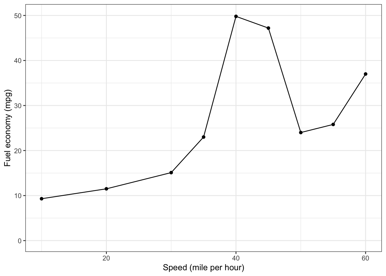
These initial data indicate that fuel economy is worse at 40 mph than at higher speeds. This goes against what you’ve heard and read about speed and fuel economy. Could something be wrong?
Answering this draws on what might be called specialist knowledge of how cars work. Gasoline is used to keep a car travelling at a constant speed, but it is also used during acceleration and saved when coasting. The shape of the fuel economy vs speed graph reflects a gasoline-consuming acceleration to around 40 mph, at which point the foot was taken off the gas momentarily, with the coasting producing the very high fuel economy. Then more acceleration to 60 mph followed again by coasting.
A schematic diagram of the factors behind fuel economy might look like Figure 8.2. Chapters @ref(causal_networks) and ?? will discuss the implications for such a network of factors, in particular how the individual arrow paths cannot be accurately quantified with just the two variables displayed in Figure 8.1.
Figure 8.2: The connections among physical quantities involved in determining fuel economy. Acceleration leads to higher speed, but lowers fuel economy. Higher speed tends to reduce fuel economy.

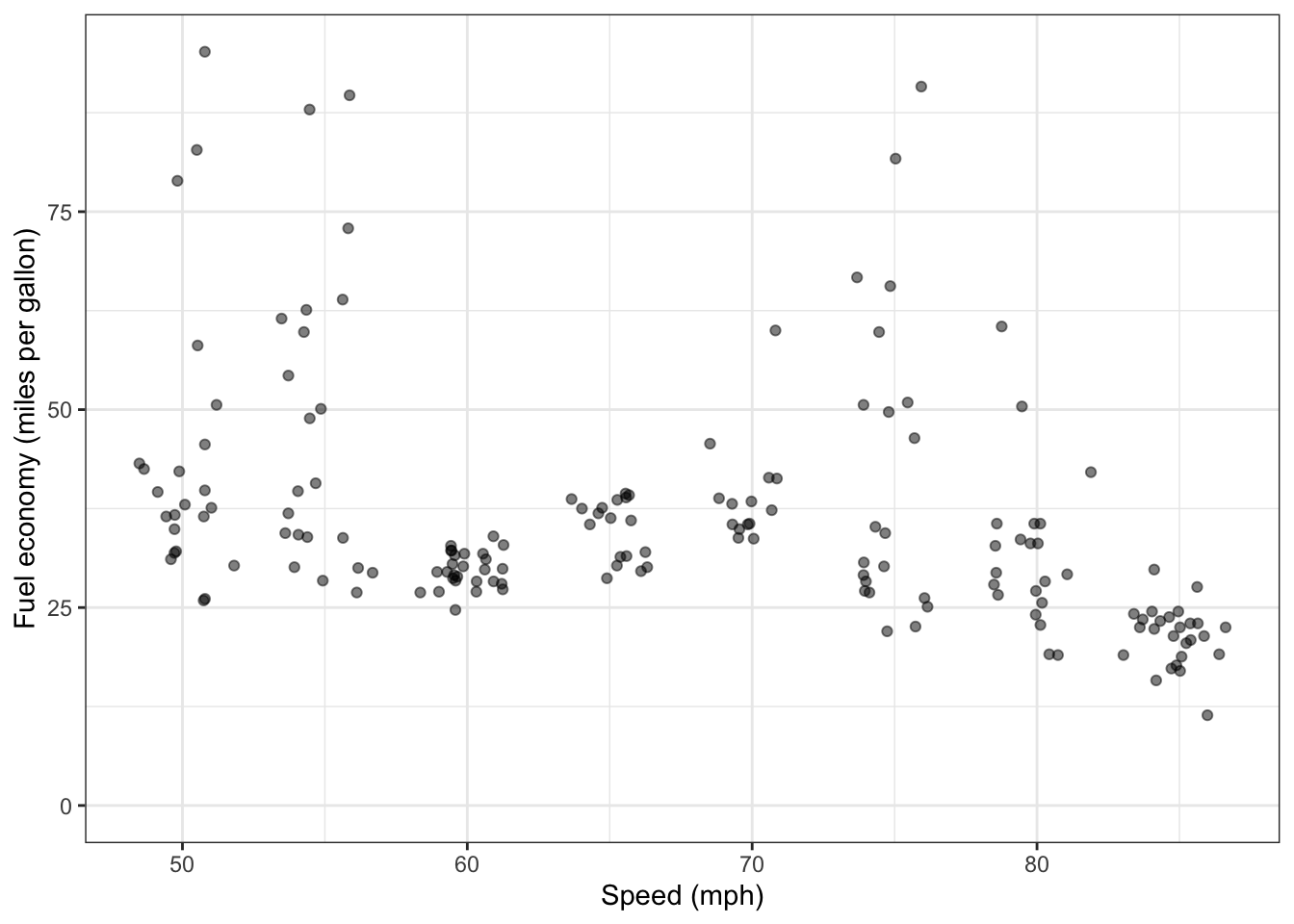
Fortunately, there’s an easy way to deal with the acceleration/deceleration effect. You amend your data-collection plan so that you’ll hold speed constant for one minute before recording data, then hold at that same speed for five minutes while you record. You also realize that even in flat areas the road can slope up or down for a mile or so. Collecting over five minutes will ensure that each data collection epoch will contain a (hopefully) representative mixture of different slopes.
Figure 8.3: “Instantaneous” fuel economy recorded while driving steadily at each of several speeds. 95% prediction intervals are shown as well as the median fuel economy. Each dot corresponds to a roughly ten-second long time span.
IV. Modeling
Now it’s time to create some mathematical representations of the situation: models. Why mathematical? For much the same reason that one designs a building using drawings and blueprints rather than bricks. Models are easy to handle and understand and modify.
Too often at this stage, people look at a statistics text to find a statistical method appropriate for the sort of data at hand. For instance, since both variables are quantitative, a standard method to apply is linear regression in which a straight line is fitted to the data as in Figure 8.4.
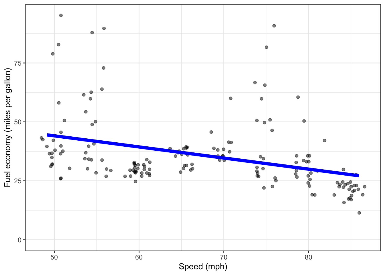
Figure 8.4: A straight-line model fitted to fuel economy versus speed.
Using a straight-line to model the data is sometimes appropriate, but not here. First, the straight line fails to go anywhere near the center value for 60, 70, and 90 mph. But more fundamentally, our purpose in constructing a model is to find the best speed for highway driving. By their nature, straight-line models cannot have a maximum in the middle of their range. Models should be suited to their purpose.
It’s easy to fall into the trap of always using a standard method (such as a straight-line model). This can lead to an inappropriate choice of methods, methods that may be “correct” but that extract misleading information from data. An image to keep to keep this warning in mind is evoked by the term cargo cult statistics. This term is used to label a too common practice which amounts to mimicking statistical procedures without understanding the actual purpose for which they were developed. The name “cargo cult” refers to “anthropological observations of Melanesian cultures that experienced a bonanza in World War II, when military cargo aircraft landed on the islands, bringing a wealth of goods. To bring back the cargo planes, islanders set up landing strips, lit fires as runway lights, and mimed communication with the oncoming planes using makeshift communication huts, wooden headsets, and the like. They went through the motions that had led to landings, without understanding the significance of those motions.” (Stark and Saltelli 2018)
Without going into details here, a more appropriate statistical technique is shown in Figure 8.5.
Figure 8.5: The relationship between fuel consumption and speed that we’ll use in the broader model. This model indicates that speed near 55 mph results in the lowest fuel consumption (of 2.5 gallons per mile), but this is almost matched at speeds of 65 to 75 mph.
Keep in mind that good fuel economy was only one of the objectives in our client’s problem, There were others such as safety, legal constraints, and the value of our client’s time. Earlier we decided how to take care of safety and the legal constraints. But we still have to figure out how to incorporate the value of our client’s time. This requires another model, for instance one that looks at the total cost of driving 100 miles, including both the cost of fuel and the value of time.
To drive 100 miles takes about 1:50 (hours:minutes) at 55 mph, about 1:32 at 65 mpg, 1:20 at 75 mpg, and 1:10 at 85. One important and reasonable modeling approach is to convert both time and gallons to money. For gallons, this is easy. Simply multiply the gallon savings by the price of gasoline. For this example, we’ll take that to be three to five dollars per gallon. (The higher figure is appropriate for Europe and Canada, the lower figure for the US.) For time, we’ve already decided that $20 per hour is a reasonable placeholder.
Table 8.1: Total cost of driving, per 100 miles, using a gasoline price of $3 / gallon and a time value of $20 per hour. Speed is miles-per-hour, gasoline is in gallons, time in hours, total cost in dollars.
| speed | gasoline | time | total_cost |
|---|---|---|---|
| 55 | 2.5 | 1.82 | 43.9 |
| 65 | 2.9 | 1.53 | 39.3 |
| 75 | 3.3 | 1.33 | 36.5 |
| 85 | 5.0 | 1.18 | 38.6 |
Table 8.1 tallies up the cost of driving 100 miles. According to the table, 75 mph is the “best” speed.
V. Assessing performance of the model(s)
Placing this section as part of a linear sequence, I, II, III, IV, and now V, is somewhat misleading. In reality, there is a back-and-forth between examining the performance of models, building models, collecting data, and gathering background information. You can see this, for instance, in the trial data in Figure 8.1, where we rejected the data collection plan because we saw a conflict between what the data we were collecting showed and what we already knew about fuel economy.
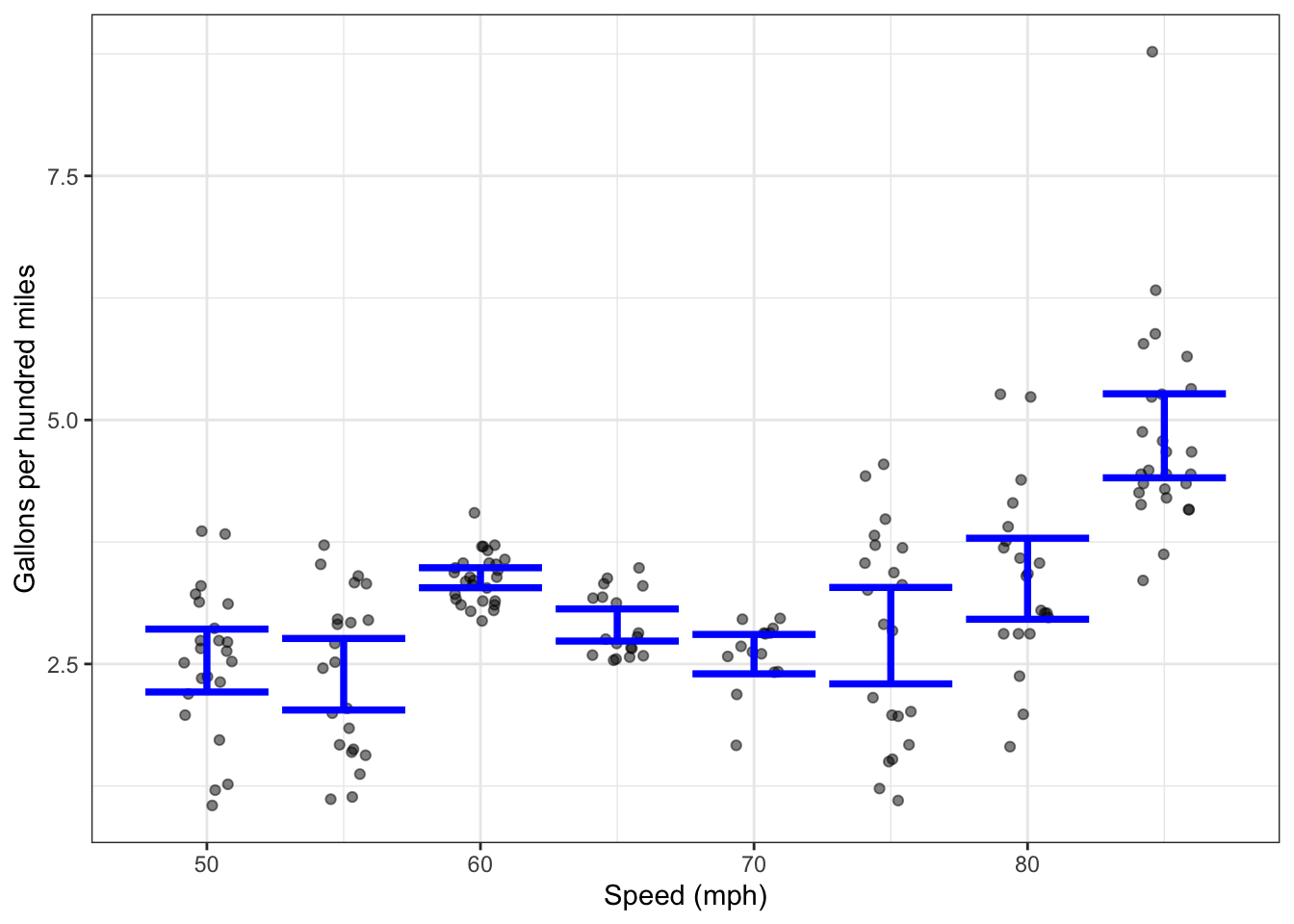
Another instance of such feedback is illustrated by the difference between the data display in Figures 8.3 and 8.5. The graph of data in Figure 8.3 shows a very broad scatter of fuel-economy readings (from 25 to 75 miles-per-gallon) even while driving the same speed. It’s good to try to understand how it could happen that driving under pretty steady conditions would lead to a variation by a multiple of 3. Figuring this out required insight and a bit of “expert” knowledge of the system under study. Recall that in gathering background information we noticed that some sources refer to “fuel economy” (miles-per-gallon) and others to “fuel consumption” (gallons-per-100-miles). These two measures are inversely related mathematically: \(\frac{100}{\mbox{mpg}} = \mbox{gallons-per-100-miles}\). It’s easy to be confused by this, but it works out that averaging the instantaneous gallons-per-100-miles (at a constant speed) gives the correct fuel consumption, but averaging miles-per-gallon doesn’t make sense. To see this, here’s a thought experiment. Suppose your engine stopped running while you were driving. The coasting car would have infinite fuel economy: \(\infty\) mpg. (Why? It’s going a distance but consuming zero gallons of fuel.) If we average fuel economy over the whole trip, that episode would bring the fuel economy to \(\infty\) mpg.
Figure 8.5 shows the data measured as gallons-per-100-miles. The spread of values at any given speed is much smaller than in Figure 8.3: instead of varying by a factor of 3, the variation from instant to instant is only about 0.5.
The interval layer in Figure 8.5 shows the average fuel consumption at each speed. The average is shown as an interval (called a 95% confidence interval) which quantifies the amount of uncertainty due to the size of the sample. (This is one of the topics to be covered in later chapters.) You can see that the intervals at different speeds overlap, which means that the data are somewhat ambiguous when it comes to concluding that fuel economy is different at different speeds.
Another way of looking at this is that the uncertainty in our knowledge of fuel consumption corresponds to an uncertainty in total cost (fuel cost plus value of time) that’s almost as big as the differences in cost we found for different speeds. This suggests that we ought to collect more data. As you’ll see in later chapters, collecting four times as much data will reduce the length of the intervals by half, which would be good enough to find out if the claimed differences in total cost are well substantiated by the data.
At this point, go back to earlier steps and fix the problem we’ve identified: not enough data. Having done that, we’re ready to move on to the next step.
VI. Communication
A coarse presentation of the results could be as simple as one sentence: “75 mph is the best speed to drive.” But think about how your client will be able to use this information.
- Will they find such an absolute statement credible? For instance, the report doesn’t describe the placeholder being used for the value of time or for the price of fuel.
- Suppose another factor comes into play, for instance the cost of meals or lodging or being asked to participate in an initiative encouraging everyone to drive slower. The “75 mph is best” short report doesn’t provide enough information to figure out how to deal with these new factors.
Your report should have enough detail so the client can figure out what factors you’ve incorporated into your conclusion – fuel use, cost of fuel, value of time – and which ones you deemed not necessary to include – safety, speed limits — and why. The client should be able easily to see how a decision to use different placeholders would affect the conclusion. Often, data scientists will provide a way for the client easily to try out different placeholders, for instance an interactive report with sliders for for fuel price and value of time.
Rather than the simple statement “75 mph is best,” say how much better it is than the alternative. For example, the difference in total cost between driving at 75 mph and either 65 or 85 is only 10%. This can give your client perspective in balancing the total dollar cost and other potential factors.
It takes judgment to translate the numbers in Table 8.1 into an answer to the question about the best speed to drive. Perhaps something like this:
As a rough guideline drive about 65 to 75 mph, but not faster than 5 mph above the posted limit. This advice applies when gasoline is about $3 per gallon and the time value of the driver and passengers is about $20 per hour. Speeds of 55 or 70 are better, considering only fuel economy, than intermediate speeds.
This recommendation, if intended to be applied to a company, would be (appropriately) rejected by the legal department. They would change it to, “It’s efficient to drive near, but not over, the posted speed limit. Make appropriate adjustments to suit weather and road safety conditions.” As a data scientist, you should be aware that there are other stakeholders in making a recommendation. Data don’t tell the whole story. In this case, the lawyer’s version is close to the target suggested by data.
As this example suggests, using data appropriately involves knowing the precise purpose for your work, having good knowledge about the workings of the system, a willingness to approximate (which sometimes involves vague considerations such as the money value of time), judgment in choosing which factors to include in your models, and a sense of the precision of conclusions and the possibilities for collecting better data. The overall outcome may well be shaped by the views of other stakeholders.
Later chapters in this book will emphasize the technical aspects of working with data, but keep in mind that purpose, judgment, and outside knowledge should always be an integral part of solving genuine problems.
References
Greene, David L. 1981. “Estimated Speed/Fuel Consumption Relationships for a Large Sample of Cars.” Energy 6 (5): 441–46. https://doi.org/https://doi.org/10.1016/0360-5442(81)90006-2.
Stark, Philip B., and Andrea Saltelli. 2018. “Cargo-Cult Statistics and Scientific Crisis.” Significance 15 (4): 40–43. https://doi.org/https://doi.org/10.1111/j.1740-9713.2018.01174.x.