Chapter 22 DRAFT: Communicating about uncertainty and risk

Example about relative and absolute risk: The risk ratios given on page 64 of the handicapped-in-school report ~/Downloads/07-23-Beyond-Suspensions.pdf. The risk ratio of 5 or 7 shows that there is an inequity. But it doesn’t show that it is an important problem in its own right.

From the same report: an example of lack of adjustment figure on page 72. The graphic gives proportions among handicapped males who were suspended by race, so the proportions add up to 100%. There is a similar display for girls, also adding up to 100%. But there’s nothing to tell us how girls and boys compare.

Second paragraph on page 67 of the report indicates that more than 70% of black students with disabilities were suspended more than once. This was picked up by news reports. But it seems that the actual rate was about 20%. See https://mail.google.com/mail/u/0/#inbox/FMfcgxwDqnkxPFHBSPtVLjlvLhkZDdnM

CAUSALITY: Page 75 of the report:

Some studies suggest that exclusionary discipline practices not only affect the individual student, but also affect their peers and the entire school environment. Removing disruptive students appears to negatively impact all student outcomes and the learning climate of the classroom.

For instance in a 2014 longitudinal study tracking approximately 17,000 students over three years, researchers found that high rates of school suspensions harmed math and reading scores for non-suspended students.429 Isolating the scores of non-suspended students, the researchers found an inverse relationship between suspension rates and test scores, meaning higher numbers of suspensions resulted in lower reading and math scores on end-of-semester evaluations. These findings suggest that high levels of suspensions “can have a very negative effect on the so-called”good apples" or rule-abiding students. The researchers found that in schools with low or average rates of suspensions, exclusionary discipline did not appear to have an effect on non-suspended students’ test scores, but the negative results appeared when schools were above average in their use of suspensions.431 University of Kentucky Professor Edward Morris posited this inverse relationship may be due to non-suspended students experiencing higher levels of anxiety and feeling disconnected from their peers who are suspended frequently, often for minor issues such as dress code violations or insubordination. These findings were consistent, even after controlling for the level of violence at the school, school funding, and student-teacher ratios. Morris stated, “When you are in a very punitive environment, you’re getting the message that the school is focusing on crime control and behavior control. Schools should really be about relationships.”

Might it be that classrooms with a lot of disruptions produce students with lower levels of learning? That’s the common sense explanation.

[JUST AN OUTLINE]

Probability is always multivariate and conditional
1. textbook examples – coin flips, dice tosses, pure exogeneity – are useful for constructing simulation models, but the probabilities of variables that matter are always conditional.
2. p(a given b) versus p(b given a) are utterly different things.
3. odds and log-odds are another way of encoding probability
4. likelihood is a technical term, so be aware!
Presentation and calculation using conditional probabilities
1. marginal probability and p(a & b) = p(a | b) p(b) = p(b | a) p(a) where p(a) is just a sum
  1. prevalence p(a) = p(a | b1) p(b1) + p(a | b2) p(b2) + … where p(b1), p(b2), etc. come from a particular sample or a statement of belief
Relative versus absolute risk
1. examples
2. ways of describing relative risk
  1. risk ratio
  2. odds ratio
  3. attributable fraction
  4. number needed to treat
Psychology of risk
1. aversion to loss
2. over-estimation of rare events
3. fright factors

In 2002, psychologist Daniel Kahneman won the Nobel Prize in economics. That may seem an odd combination of academic fields, but Kahneman’s work, much of which was done with his close colleague Amos Tversky, highlighted the ways that intuitive reasoning, rather than careful calculation, govern human processes for judgement, making decisions, and assessing risk. (See Kahneman (2011).) People are emotional creatures: they like and dislike, they are influenced by first impressions and irrelevant “anchors”, they impose an exagerated emotional coherence that forces into alignment ideas like value and risk.

Use Titanic table in Small-data chapter to illustrate risk ratio and odds ratio.

Not p-values: - ASA editorial March 2019 - Nature article March 2019

From Tversky and Kahneman (1974)

“Statistical principles are not learned from everyday experience.”

“Although the statistically sophisticated avoid elementary errors, such as the gambler’s fallacy, their intuitive judgments are liable to similar fallacies in more intricate and less transparent problems.”

22.1 10-year risk of disease

Present this entire table and discuss whether the risk of lung cancer is the issue or whether it is all-cause mortality.

https://www.ncbi.nlm.nih.gov/pmc/articles/PMC3298961/figure/fig2/

What do you think about the format shown in https://www.ncbi.nlm.nih.gov/pmc/articles/PMC6010924/#bb0130 (Figure 4) for comparing lifetime risk to risk in any age decade. Maybe this is a better way than Woloshin et alia (2008) to put 10-year risk in the context of lifetime risk. Can you get a similar graph for breast cancer?

22.2 Odds ratios

Return to the Schrek et al. (1950) example in 026-Bayes.Rmd and show that the odds ratio comparing lung cancer in smokers and non-smokers is the same as the odds ratio comparing smoking in lung cancer and non-lung cancer.

22.3 Probability

Relative frequencies.

Classifier output.

Subjective probability.

22.4 Conditional probabilities

Remember the sensitivity / specificity distinction made in the HBC example in the chapter on classifier error. Let’s return to that.

We built a toy classifier to identify people at high risk of high blood pressure. The classifier took the form of a model, with age, sex, and [whatever] as inputs. The categorical outputs have the levels “will develop high blood pressure” and “will not”. Given inputs, the classifier generates an output in the form of a probability assigned to each level, for instance, “the probabiility that the person will develop high blood pressure given age = 60, sex = M, and so on”.

Recall the definition of probability given in Chapter @ref(summarizing data): a probability is a number between zero and one. The classifier output is in the form of a probability, but it is not necessarily a good estimate

Now the wrench in the works. That probability is valid only for the population from whom the training data was taken. It’s tempting to think that this population is the HBC clients, since the HBC database was used to extract the training (and testing) data. But not really. Half of the people in the training data are people who have developed high blood pressure. These are not representative of the overall population of clients because it’s not the case that half the people in the overall population have high blood pressure. Similarly, half the testing data consists of people matched to the high-blood pressure individuals who have not developed high blood pressure. This half might be different from the overall population in many ways, since it is matched to the high blood pressure individuals already selected.

What you’re actually interested in is the probability for a person from the overall population that he or she will go on to develop high blood pressure. In order to find this, we’re going to need to convert the classifier output into a probability reflecting the overall population.

Scientific knowledge: sensitivity and specificity

Assumption: Incidence of high blood pressure over the next five years.

Desired probability: Given a positive result, what’s the probability of developing high blood pressure.

CHANGE THE classifier-example to be some already existing (but undetected) trait. THEN USE THE retrospective cohort method in the study design chapter.

, it assigned a probability

22.5 Describing changes in risk

Percent versus percentage points in talking about changes in risk.

Odds ratios, risk ratios, attributable fraction, number needed to treat, …

22.6 Quantifying cost

lives saved, life-years saved, QALY

22.7 Example: Risk of dementia

See article at https://www.bbc.com/news/health-46155607 about a study that identifies a 50% increase in risk of dementia in a group of people. But is this actionable?

22.8 Example: Too fat or too thin?

See article at https://www.bbc.com/news/health-46031332 for optimal BMI to reduce mortality.

22.9 Example: Risk of breast cancer

A randomly selected woman in the US, age 30+, has about a 2.3% chance of developing breast cancer sometime in the next 10 years. (More precisely, this is the chance of being diagnosed with breast cancer.) This 2.3% number can be thought of as the output of a no-input classifier. Using explanatory variables as inputs changes the result. For instance, an extremely important factor in many medical situations is age. According the the US National Cancer Institute (NCI), a classifier with age as an input would look like this:

Age	Probability of being diagnosed with cancer in the next ten years
30	0.44% (or 1 in 227)
40	1.47% (or 1 in 68)
50	2.38% (or 1 in 42)
60	3.56% (or 1 in 28)
70	3.82% (or 1 in 26)

Of course, it’s possible to build classifiers with more inputs than age. One such classifier offered by the NCI, the Gail model includes these inputs:

age
race/ethnicity
age at first menstrual period
age at birth of first child (if any)
whether the woman’s close relatives (mother, sisters, or children) have had breast cancer
whether the woman has ever had a breast biopsy
whether the woman has a medical history of breast cancer
whether the woman has a mutation in the BRCA 1 or BRCA 2 gene of the type associated with higher risk for breast cancer.

For example, according to the Gail model, a 55-year-old, African-American woman who has never had a breast biopsy or any history of breast cancer, who doesn’t know her BRCA status, and whose close relatives have no history of breast cancer, whose first menstrual period was at age 13 and first child at age 23 has a 1.4% probability of developing breast cancer over the next five years. In comparison, if more than one of the woman’s close relatives has a history of breast cancer, the model output is 3.5%.

You can think of the Gail model as a classifier. It takes as inputs information that many women have available and produces one of two outputs: “You will be diagnosed with cancer in the next five years” or not. As appropriate for a classifier, the actual output is a probability of each of these two levels. We call the probability a risk.

An important instrument for detecting breast cancer is mammography. Mammography involves taking an X-ray picture of a breast and examining the picture for the unusually dense tissue or calcifications which are a sign of cancer. Medically oriented people don’t usually think of mammography as a classifier. Instead, they appropriately call it a test, which gives an indication of … well, what? The outcome of mammography is not a diagnosis of breast cancer; the output levels are not cancer vs no cancer. Instead, the outputs of mammography are the abstract labels “positive” or “negative.” A negative outcome is interpreted to mean that no further follow-up is needed at present. A positive outcome generally leads to more intensive and invasive testing, such as a biopsy.

Most women who undergo a mammogram do not have any signs or symptoms of breast cancer. The mammogram is a particular kind of test called a screening test.

One way in which mammography is not a classifier is that the output is not stated as a probability of each outcome. Instead, the output is the labels themselves: “positive” or “negative.”

For the sake of discussion, let’s imagine what mammography would look like as a cancer-risk classifier. Different classifiers could be constructed that take into account other stratifying variables such as those used in the Gail model, but let’s consider a one-input classifier taking just the mammography results and nothing else as input and that women.

For women aged 50+, the 3-year risk of developing cancer is about 2%. A negative mammogram would correspond to a risk of cancer just under this 2%. In contrast, a positive mammogram indicates a risk of cancer of about 16%. (Mammography at age 50+ is consistent with many medical organizations’ guidelines. For younger women, mammography is generally not specifically recommended, although it is not actively discouraged. For women in their 30s, the numbers are substantially different. A positive mammogram for this group corresponds to a risk of cancer of about 1%.)

Some readers may be surprised to hear that a positive mammogram (for women 50+) corresponds to a cancer risk of 16%. The misconception that a positive mammogram means it’s almost certain that the woman has breast cancer is wide-spread, even among physicians. It’s hardly reasonable to think that 16% is high enough to be a diagnosis for cancer, but since mammography is (properly) used only to prompt further investigation, that low probability is acceptable.

Should the results of mammography be reported as a probability or, as is actually done, as positive vs negative? Certainly, any probability calculation should take into account other factors such as those in the Gail model. And, for statisticians and policy makers (and the readers of this book) a probability is the better format. That might not be the case for the general public, however.

22.10 Example: Does mammography help?

Emphasize that this is controversial and that there are other interests at play than overall public health outcomes.

See “Screening for Breast Cancer An Update for the U.S. Preventive Services Task Force” available here. There’s no detectable reduction in overall mortality, but there is in breast cancer mortality. Note also the Number needed to treat for biopsy (given positive imaging) reported near the end.

Life-years saved

Need to look at overall mortality, not survival. Problem of over-diagnosis. See overall risk of dying from cancer

Incidence goes up by about 25% from 1980 to 1990. Why? Over-diagnosis? Incidence doesn’t change for men over that period.

Mortality goes down by about 35% starting about 1995 to 2014. Better treatment? Other sources of death? Mortality doesn’t improve for men.

Survival rate goes up over the decades for both whites and blacks: See https://seer.cancer.gov/archive/csr/1975_2014/results_merged/topic_survival.pdf table 4.13. Goes from about 75% in the mid-1970s to 91% around 2010.

QUESTION: Is the survival data consistent with the mortality data. In survival rates, the denominator is “women who have been diagnosed with cancer,” while in mortality the denominator is “all women.” Obvious answer: Yes: survival goes up so mortality goes down. But let’s look at it quantitatively. 25% of those diagnosed die (within 5 years) in the 1970s. By 2010, only 9% die. If incidence were stable, this would mean that 5-year mortality in 1970s to 2010 ought to go down by more than 60% (death rate is 25 per 100 in 1970s and 9 per 100 in 2010). What can cause the difference?

Overdiagnosis: more women who have a condition diagnosed as cancer but not actually lethal are included in the denominator “# diagnosed with cancer.”
- suppose in 1970s, 50% of diagnoses are over-diagnosis. Of the remaining 50%, one-half die, giving overall survival of 75%.
- suppose in 2010, 75% of diagnosis are over-diagnosis. (This is consistent with an increase in incidence of about 25% due to over-diagnosis.) Of the remaining 25% of diagnoses, 36% will die, leading to an overall survival of 91%.
- the decrease from 50% to 36% death rates is consistent with mortality going down by about 35%
Lead time bias: But that can’t plausibly explain a reduction from 25% to 9%.

22.11 Example: Predictive modeling of diabetes

One of the ways that we talk about the possible onset or risk of disease is through risk factors. For instance, smoking is a well known and very strong risk factor for lung cancer and emphysema. Risk factors are observable traits or conditions that can be used to predict the onset of a disease. One way to identify and quantify risk factors is to build a predictive model from a data frame that contains the measurements of potential risk factors along with the eventual outcome for many people. As an illustration, consider the National Health and Nutrition Evaluation Survey data. NHANES records which people have diabetes as well as many other variables such as age, height, weight, and so on.

To construct a prediction model, you can condition the outcome on whatever explanatory variables you choose. Here, we’ll look at a model that bases the prediction of body mass index (BMI), income, age, sex, and whether a person has an education beyond the 8th grade.

Figure 22.1: A schematic drawing of a prediction model for diabetes. You specify values for the input variables and, using some mathematics we have not yet covered, the output is generated.

A schematic drawing of a prediction model for diabetes. You specify values for the input variables and, using some mathematics we have not yet covered, the output is generated.

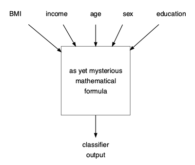
In Chapter ?? we’ll introduce methods for constructing classifiers with quantitative inputs (e.g. BMI, age). For now, note that since the classifier is implemented as a computer program, you can make predictions even without knowing the details of how the classifier was constructed. You just have to evaluate the mathematical formula at the core of the classifier: provide the relevant inputs to the software implementing the classifier and observe the classifier’s output.

Let’s look at some example predictions from the classifier:

Table 22.1: Inputs to the classifier shown in Figure 22.1, along with the classifier output in the form of probabilities of each possible outcome.

age	sex	income	education	BMI	prob_diabetes	prob_no_diabetes
40	male	1.5	8th grade	42	0.18	0.82
61	male	> 5	college grad	61	0.59	0.41
75	female	3.5	high school grad	34	0.41	0.59

22.12 Example: Red meat and colon cancer

Link to article

Red and processed meats intake was associated with increased colorectal cancer risk. The summary relative risk (RR) of colorectal cancer for the highest versus the lowest intake was 1.22 (95% CI = 1.11 - 1.34) and the RR for every 100 g/day increase was 1.14 (95% CI = 1.04 - 1.24)…. The associations were similar for colon and rectal cancer risk. When analyzed separately, colorectal cancer risk was related to intake of fresh red meat (RR for 100 g/day increase = 1.17, 95% CI = 1.05 - 1.31) and processed meat (RR for 50 g/day increase = 1.18, 95% CI = 1.10 - 1.28). Similar results were observed for colon cancer, but for rectal cancer, no significant associations were observed.

Conclusions: High intake of red and processed meat is associated with significant increased risk of colorectal, colon and rectal cancers. The overall evidence of prospective studies supports limiting red and processed meat consumption as one of the dietary recommendations for the prevention of colorectal cancer.

How to interpret a risk ratio of 1.22? Is it for cancer of any type, or just colorectal cancer.

See lifetime probability of developing and of dying from cancer. Roughly a 4.5% chance of developing colorectal cancer. Reducing this by 30% would result in a 3.1% chance of developing colorectal cancer. Attributable fraction of colorectal cancers: 43%.

Lifetime risk of all cancers: about 38%. Reduction by eliminating red meat: 1.4 percentage points. Attributable fraction: 4%.

PERHAPS AS AN EXERCISE:

Compare this graph to the interpretation found in the abstract

Figure 22.2: From figure 3 of the PLOS article

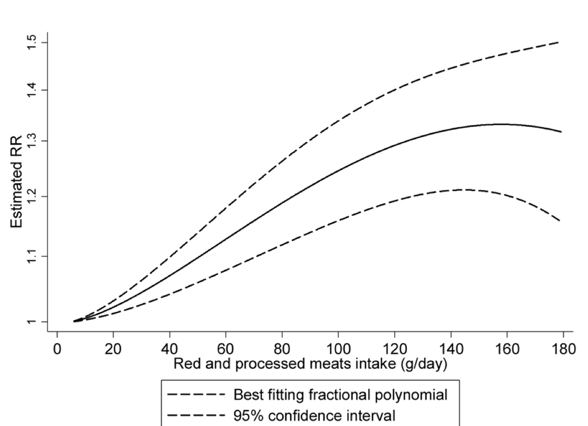
The confidence band is so broad that the statement about a plateau seems unjustified. A straight line fits nicely within the confidence band.

Non-linear dose-response meta-analyses revealed that colorectal cancer risk increases approximately linearly with increasing intake of red and processed meats up to approximately 140 g/day, where the curve approaches its plateau.

22.13 Driving at night

Vehicle occupant fatalities per vehicle mile:

Nationwide almost half (49%) of passenger vehicle occupant fatalities occur during nighttime. This, coupled with the fact that approximately 25 percent of travel occurs during hours of darkness, 2.3 the fatality rate per vehicle mile of travel is about three times higher at night than during the day. Passenger Vehicle Occupant Fatalities by Day and Night https://crashstats.nhtsa.dot.gov/Api/Public/ViewPublication/810637

The causal diagram behind taking the 2.3 risk ratio at face value is

driving at night $\rightarrow$ risk of fatality

But a more nuanced diagram is

Nighttime  -> driving difficulty ->         )
  |                                         )
  v                                         )
Social factors -> alcohol use ->            ) risk of fatality
& demographics -> speeding  ->              )
               -> not wearing seat belt ->  )

See statistics here. Try to estimate direct effect of nighttime increase in driving difficulty with the risk of fatality.

22.14 COPMAS

A tool called COMPAS (Correctional Offender Management Profiling for Alternative Sanctions) is used for predicting whether an arrested suspect is likely to re-offend if released while awaiting trial. Such a tool is potentially useful to everyone involved. The arrested person is much better off not being in jail while waiting for a trial: he or she can keep their job, help their family, and avoid exposure to the risky conditions of jail. The state can save money, since it doesn’t have to house and feed the accused. On the other hand, if the suspect is going to commit a crime while on release, it makes sense not to release them.

Whether COMPAS is helpful or hurtful depends on how precise its predictions are. If the predictions are highly reliable, then common sense recommends using it. To know whether to use COMPAS predictions, judges and other decision makers need to know how precise the predictions are. And to know this, they need to understand how to describe uncertainty in a meaningful way. With COMPAS, the authorities had the published results of a research study. The abstract of the published report summarizes the results:

[This] article describes the basic features of COMPAS and then examines the predictive validity of the COMPAS risk scales by fitting Cox proportional hazards models to recidivism outcomes in a sample of presentence investigation and probation intake cases (N = 2,328). Results indicate that the predictive validities for the COMPAS recidivism risk model, as assessed by the area under the receiver operating characteristic curve (AUC), equal or exceed similar 4G instruments. The AUCs ranged from .66 to .80 for diverse offender subpopulations across three outcome criteria, with a majority of these exceeding .70. (Brennan, Dieterich, and Ehret 2008)

So is COMPAS helpful or hurtful? Could you argue for or against its use based on these results? Could you even tell whether the information from the study is useful for making a fair and informed judgement of whether to use COMPAS? And what should be make of this finding from the investigative journalism organization Pro Publica:

Black defendants were often predicted to be at a higher risk of recidivism than they actually were. Our analysis found that black defendants who did not recidivate over a two-year period were nearly twice as likely to be misclassified as higher risk compared to their white counterparts (45 percent vs. 23 percent). (Larson et al., n.d.)

22.15 Notes

CIA notes on perception of probabilities: https://www.cia.gov/library/center-for-the-study-of-intelligence/csi-publications/books-and-monographs/psychology-of-intelligence-analysis/art15.html

Exercise: From Hill-1937a-WA-VIII.pdf Table VII, ask students to calculate risk ratios, odds ratios.

22.16 Weasel words and effect size

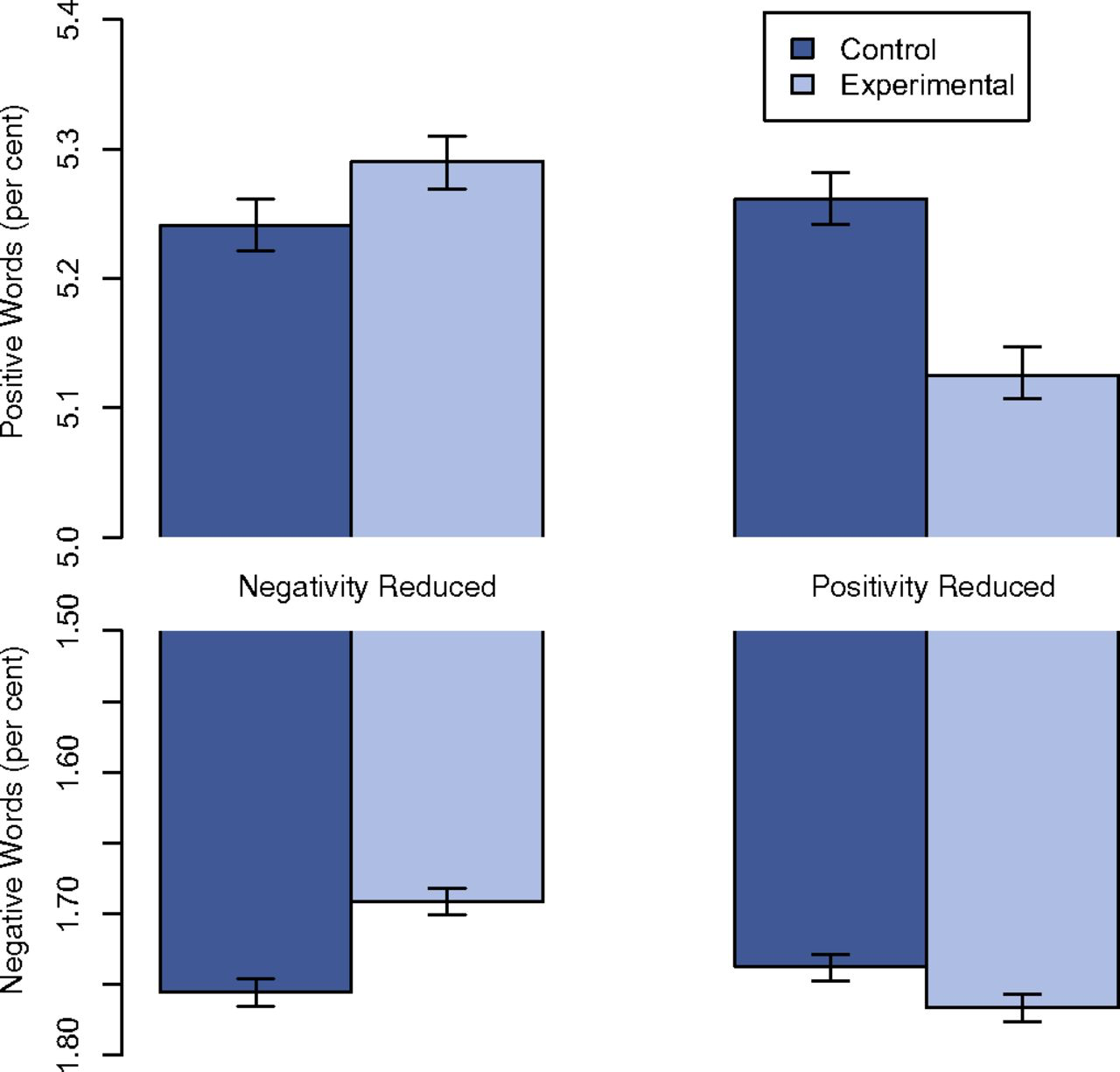
Figure 22.3 shows the output of an experiment (Kramer, JE Guillory, and Hancock 2014) that suppressed a fraction of Facebook subscribers’ news-feed posts that expressed “positive” sentiment and examined how the subscriber’s own use of positive and negative words changed. (A similar experiment was done suppressing news-feeds with “negative” sentiment.)

Figure 22.3: Use of positive and negative words by Facebook subscribers changed when the subscriber’s news feed was depleted of positive posts.

The book Hello, World (Fry 2018) described the experiment and its results:

[An] experiment run by Facebook employees in 2013 manipulated the news feeds of 689,003 users in an attempt to control their emotions and influence their moods. The experimenters suppressed any friends’ posts that contained positive words, and then did the same with those containing negative words, and watched to see how the unsuspecting subjects would react in each case. Users who saw less negative content in their feeds went on to post more positive stuff themselves. Meanwhile, those who had positive posts hidden from their timeline went on to use more negative words themselves. Conclusion: we may think we’re immune to emotional manipulation, but we’re probably not.

You can refer to Figure 22.3 to quantify the change in the use of positive words. When negative content was suppressed compared to control, positive word use increased from 5.25% of all words to 5.29%. This corresponds to a difference of 0.04 percentage points, or a ratio of 1.008. Any way you look at it, this change is small. Would any human reader be able to detect a change in emotional state signaled by a change from 125 positive words to 126 positive words out of 2500 words altogether.

Since the topic is emotional manipulation, it’s worth pointing to the impression that might be created by the above paragraph. The word “more” is vague and imprecise; the color of the paragraph is set by words like “control their emotions”, “hidden”, “emotional manipulation.”

Read that paragraph again carefully and try to estimate what was the effect size. As always, an effect size is a ratio: the change in output divided by the change in input. One of the measured outputs is the fraction of words posted by the participant that are “positive.” Another was the fraction of words posted that are “negative.” The input is the change in the fraction of news-feed posts containing positive words. (Another branch of the experiment suppressed “negative” posts.)

The output is not described in detail but we are told the suppression of negative posts produced “more positive stuff”, whereas the suppression of negative posts produced “more negative words.”

Similarly, the change in input is not detailed: “suppressed any friends’ posts that contained positive words”. Does “any” mean “all”? Were even weakly positive words suppressed: “ok”, “nice”, “good”? Or did the suppressed post have to be over-the-top with glee: “ecstatic”, “fantastic”, “brilliant”, “supurb”? It turns out that the “difference [in output] amounted to less than one-tenth of one percentage point.”

Were the subjects of the experiments really victims who were deprived over an extensive period of any positive news from their friends? Or was merely an occasional post suppressed? An effect size quantifies both the change in output and the change in input. “More” is not an effect size.

A report of the experiment summarized in the quote that begins this section was published in 2014 with the title “Experimental evidence of massive-scale emotional contagion through social networks.” (Kramer, JE Guillory, and Hancock 2014) What did the authors intend to convey by using the word “massive?” Before reading on, think about the possibilities and the impression created by the title.

A more accurate title would have been, “Social media experiment conducted on a massive-scale shows a small influence of ‘emotional contagion’.” The experiment involved about 690,000 (unwitting) participants.2121 The failure to secure the informed consent of the participants resulted in an “editorial expression of concern” by the journal. The editors wrote: “Obtaining informed consent and allowing participants to opt out are best practices in most instances under the US Department of Health and Human Services Policy for the Protection of Human Research Subjects (the “Common Rule” [a US federal government “Policy for the Protection of Human Subjects”]). The intervention in the experiment was to suppress a fraction of posts that would otherwise have appeared on the participant’s news feed, and to examine the extent to which the participant’s own subsequent postings used positive and negative words. A similar experiment involved suppressing a fraction of negative posts destined for the participant’s news feed.

An effect size in the sense of this chapter is a comparison of the change in the output (say, fraction of positive words used by the participant) to the change in the input (say, fraction of news feed posts with positive words).

In informal English usage, a “weasel” is a person who is sneaky, deceitful, and cunning. Words that are used in a way to create a false impression that something definite has been said are sometimes called weasel words. It’s not necessarily the case that the person using a weasel word is being intentionally deceitful. People can believe that the words have a definite meaning when, in fact, they provide nothing more than an impression.

It’s helpful to keep an eye out for weasel words and to ask, when they are sighted, what is the missing numerical quantity. Here are a few weasel words together with the style of numerical statement that would provide an informative sense of the quantity being expressed.

Weasel word	Examples of specific quantity
often	Daily, Yearly, 30% of the time
inexpensive	$1.50 for a sandwich, $3 billion for an aircraft carrier
regularly	Halley’s comet comes every 76 years
could	One time in a thousand
some	around 3% of people
effective	reduced attacks by 37%
safe	one death per 17 million passenger miles
risky	one injury per 500 jumps
increasing	by 2% per year
significant	increases the probability of success by 10 percentage points

The word “significant” is a weasel word that, regretably, has been constructed collectively by the statistics community. It has a technical meaning in statistics that often does not correspond to its everyday meaning. So a phrase like “the study found a significant decrease in the risk of pancreatitis,” does not necessarily mean that the study found a clinically meaningful effect. We’ll return to the many problems with “statistical significance” in Chapter @ref(false_discovery).

Words like “skyrocket,” “surge”, and “plummet” are found frequently in news reports. If a reporter knows that some quantity has increased, he or she should be able to quantify the change, even if roughly. Does unemployment skyrocket if it goes from 4.8 to 5.2 percent? Does the stock market plummet when it’s down 3% for the day? What is the boundary between “often” and “occasionally?”

A CIA essay on Weasel words: https://www.cia.gov/library/center-for-the-study-of-intelligence/csi-publications/books-and-monographs/sherman-kent-and-the-board-of-national-estimates-collected-essays/6words.html

References

Brennan, Tim, William Dieterich, and Beate Ehret. 2008. “Evaluating the Predictive Validity of the Compas Risk and Needs Assessment System.” Criminal Justice and Behavior 36 (1). https://jpo.wrlc.org/handle/11204/1123.

Fry, Hannah. 2018. Hello World: Being Human in the Age of Algorithms. W.W. Norton.

Kahneman, Daniel. 2011. Thinking, Fast and Slow. Farrar, Straus,; Giroux.

Kramer, Adam, JE Guillory, and JT Hancock. 2014. “Experimental Evidence of Massive-Scale Emotional Contagion Through Social Networks.” Proceedings of the National Academy of Sciences 111 (24): 8788–90. https://doi.org/10.1073/pnas.1320040111.

Larson, Jeff, Surya Mattu, Lauren Kirchner, and Julia Angwin. n.d. “How We Analyzed the Compas Recidivism Algorithm.” Pro Publica. https://www.propublica.org/article/how-we-analyzed-the-compas-recidivism-algorithm.

Schrek, Robert, Lyle A. Baker, George P. Ballard, and Sidney Dolgoff. 1950. “Tobacco Smoking as an Etiologic Factor in Disease. I. Cancer.” Cancer Research 10: 49–58.

Tversky, Amos, and Daniel Kahneman. 1974. “Judgements Under Uncertainty: Heuristics and Biases.” Science 185 (4157): 1124–31.

Woloshin et alia, Steven. 2008. “The Risk of Death by Age, Sex, and Smoking Status in the United States: Putting Health Risks in Context.” Journal of the National Cancer Institute 100 (12): 845–53. https://www.ncbi.nlm.nih.gov/pmc/articles/PMC3298961/.