Chapter 21 DRAFT: Adjustment
JUST NOTES
- Comparing like things
- Assembling conditional probabilities into a whole, e.g. survey weighting
More things…
- Making meaningful comparisons: stratify and compare strata
- Add up the comparisons for each strata with an agreed-upon, standard weight for each strata.
21.1 Weighting in polls
https://www.nytimes.com/2018/09/06/upshot/live-poll-explainer.html see also https://www.nytimes.com/2018/09/06/upshot/midterms-2018-polls-live.html
21.2 Minimum wage example
See Figure 21.1.
21.3 Comparing to an index
Case mortality from Hill-1937a-WA-III.pdf (perhaps for exercise).

21.4 Mismeasure of man
As described in Gould (1996) (pp. 87-99), in the 19th century, racist assertions of superiority were tied to measurements of brain size, with so-called superior races having, on average, the largest brains. There’s no justification for the association of superior intellect with brain size. People of short stature tend to have smaller brains than those of large stature, females tend to have smaller brains than males. In assembling the averages by race, no attempt was made to adjust for the stature of individuals. The claimed differences between the races was substantially the product of the samples used having different mixtures of small- and large-statured people included.
21.5 Age adjustment
A specific example in a context that’s easy to understand. Mortality rates among countries.
Mortality rates: adjusting for age
Cancer rates: adjusting for age
See https://ourworldindata.org/causes-of-death for many death-rate stats.
21.6 Adjustment for covariates
21.7 Seasonal adjustment
Separating out known sources of variation from unknown ones.
21.8 Example
Age-adjusted incidence and mortality rates by year of diagnosis, see https://seer.cancer.gov/archive/csr/1975_2014/results_merged/topic_annualrates.pdf tables 4.5 and 4.6
21.9 More details
From conditioning to correlation: p(xy) = p(y | x) p(x) = p(x | y) p(y)
Use tilde instead of |. So p(xy) = p(y ~ x)p(x)
THIS NEXT CHUNK ISN’T WORKING. FIX IT
story_A <- list(C ~ 0,
                A ~  - C,
                Y ~  A + 4*C)
set.seed(88)
A_data <- acy_sim(story = story_A, samp_n = 1000, numerical = "Y")
set.seed(88)
B_data <- sem_sim(story = story_A, samp_n = 1000)
condition_plot(~ Y_num, data = A_data, alpha = 0.05)
condition_plot(~ Y, data = A_data, alpha = 0.05)
condition2_plot(Y ~ A, data = A_data, alpha = 0.05)
condition2_plot(Y ~ C + A, data = A_data, alpha = 0.05)
summary(glm(Y ~ A, data = A_data, family = binomial))
summary(glm(Y ~ A + C, data = A_data, family = binomial))
odds2_plot(Y ~ A, data = A_data)
odds2_plot(Y ~ A + C, data = A_data)
21.10 Example: The minimum wage, ceterus paribus, and mutatis mutandis
Throughout the US, there is debate about increasing the minimum wage. Figure 21.1 shows the minimum wage mandated by US Federal law over the years since 1938. The graph shows that the minimum wage has been going up over the decades. Proponents of an wage increase point out that this basic pattern is misleading. They argue, reasonably enough, that inflation over the decades has reduced the value of money. One way to look at the minimum wage, all other things being equal, is to adjust it for inflation. We’ll discuss adjustment in Chapter ??, but for now it suffices to point out that an accepted technique for adjusting for inflation is to present the wage in constant dollars is shown in 21.1. The adjusted wage (dashed line) in 1983 constant dollars. The wage presently is about 25% below its constant-dollar value during the 20-year span from 1960 to 1980.
Figure 21.1: The US Federal minimum wage over the last century shown in nominal dollars. The dashed line gives the wage adjusted for inflation by the consumer price index.
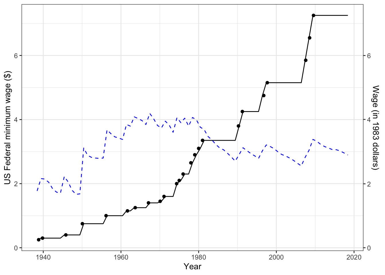
Opponents of an increase in minimum wage do not dispute the use of constant dollars in tracing the minimum wage over the years. That is, they also see the virtues of considering the wage ceterus paribus, that is, “all other things being equal.” They argue, however, that one goal in setting the minimum wage is to provide ready gainful employment for people who don’t yet qualify for a higher-paying job. The opponents reasonably argue that looking at things ceterus paribus, is misleading, because the real-world effect of an increased minimum wage has consequences beyond the wage itself. In particular, a higher minimum wage might cause employers to hire less, replacing, wherever possible, low-trained employees with automation. So while it makes sense to adjust for inflation, the impact of a minimum wage increase has to be seen ****mutatis mutandis**** – not holding everything else constant but letting some things (e.g. hiring) change as they will in response to the minimum wage increase.
A basic claim in economics is that, ceteris paribus, a higher price corresponds to a lower demand. That doesn’t resolve the question of the minimum wage. For instance, any decrease in hiring might be so small that, taking into account the higher wage, the group of people currently earning the minimum wage might see an increase in total income: fewer hours, but at a higher wage.
How would you determine the extent to which a higher minimum wage reduces the number of jobs available? It can be tempting to do this by comparing unemployment rates in cities with different minimum wages. Do high-wage cities have high unemployment? Before jumping into the data, think carefully about the choice of explanatory variables for stratification. What could you use for stratification to take into account the theory that high-wage cities attract workers from other areas, thereby raising unemployment? Or, it might be that a high cost of living creates a shortage of workers, greasing the political skids to provide political consensus around having a high minimum wage.
Many of the disputes about data used to inform social policies are about which explanatory variables to use for stratification (ceteris paribus) and which explanatory variables to ignore (mutatis mutandis).
References
Gould, Stephen Jay. 1996. The Mismeasure of Man. Revised and expanded. W.W. Norton.