Null_sim <- datasim_make(
  y <- rnorm(n),
  x <- rnorm(n)
)29 Hypothesis testing
Q: Why do so many colleges and grad schools teach p = 0.05?
A: Because that’s still what the scientific community and journal editors use.
Q: Why do so many people still use p = 0.05?
A: Because that’s what they were taught in college or grad school.
From a 2014 talk by George Cobb (1947-2020)
Lesson ?sec-Bayes introduced Bayes’ Rule, a mathematically correct formula for combining prior belief with new data in order to calculate the appropriate level of posterior belief . Statistical pioneers in the early 20th century strongly disparaged the use of Bayes’ Rule. This had nothing to do with the mathematics of Bayes’ Rule, and everything to do with the statisticians’ views of proper scientific method. In particular, the statisticians argued that science ought to be based entirely in data and therefore objective, that is, independent of individual researchers. They pointed out that the prior used in Bayesian calculations is subjective, that is, depending on the researcher’s beliefs before data have been recorded.
One of these statistical pioneers, Ronald Fisher (1890-1962), introduced in the 1920s methods of hypothetical thinking in which a prior has no role. Fisher’s “significance tests” became a leading application of statistical method and remains the core method covered in conventional introductory textbooks where it is called “statistical inference” or “hypothesis testing” or, more specifically, “Null hypothesis testing.”
For decades, statisticians have pointed out that, in practice, hypothesis testing is often mis-applied and misinterpreted. In the 21st century, some statisticians have blamed hypothesis testing for leading to a “crisis of credibility” in science. Although the notion that science ought to be “objective” is attractive, the hypothesis-testing framework does not hold up well under the pressure of the massive research enterprise that has emerged since Fisher’s day.
Despite these problems, or perhaps because of these problems, understanding hypothesis testing is a basic part of scientific and statistical literacy. This include having a firm grasp on opposing themes: the ways hypothesis testing is useful; and the reason why hypothesis testing is a source of fundamental problems in interpreting scientific research.
“Significance” testing
We start with the earliest and still very common form of hypothesis testing, what Fisher called “tests of significance.” Another name is Null hypothesis testing or NHT for short. In understanding NHT, it is essential to keep in mind that there is only one hypothesis involved. This contrasts with Bayesian inference, which always involves at least two competing hypotheses.
Another essential contrast between NHT and Bayes relates to the format of the outcome. The posterior probability in Bayes is a number that indicates the relative belief of the competing hypotheses. In NHT, the outcome is restricted to one of two possibilities:
Allowed NHT outcomes
- “Reject the Null hypothesis.”
- “Fail to reject the Null hypothesis.”
Neither of the two allowed NHT outcomes is a number; neither is a Bayes-style quantification of level of belief in the Null hypothesis; neither states any probability that the Null hypothesis is true. Indeed, the Frequentist attitude holds that it’s no legitimate to talk of the “probability of a hypothesis.”
For those who have previously studied NHT
The reader who has already studied NHT may be confounded by the claims of the previous two paragraphs.
Claim 1: There is only one hypothesis involved in NHT. The reader may well ask, “What about the alternative hypothesis ?”
Claim 2: There is no numerical outcome of NHT. In disputing this claim, the reader may wonder, “What about the p-value ?
The alternative hypothesis was is not part of NHT, but instead is part of a different approach, which we will call NP and will discuss later, when the fundamentals of NHT have been understood.
The p-value is part of an intermediate calculation often used in conducting NHT, but is not a proper outcome of NHT. However, many people are intuitively dissatisfied with the NHT outcome, and improperly use the intermediate calculation to make NHT seem more Bayes-like.
The single hypothesis involved in NHT is, as the name NHT suggests, the Null hypotheses . Using the context of statistical modeling, with its framework of the response variable, explanatory variables, and covariates, the Null hypothesis can be stated plainly:
Null hypothesis: There is no relationship between the explanatory variable(s) and the response variable, taking into account any covariates.
In the spirit of hypothetical thinking, to conduct an NHT, we examine what our summary statistics would look like if the Null were true.
Suppose we set aside, just for the purposes of discussion, the consequences of sampling variation . Then the Null hypothesis—the claim of “no relationship”—would lead to the coefficient(s) on our explanatory variable(s) being exactly zero.
In the presence of sampling variation, however, it is a fool’s errand to test whether a coefficient is exactly zero. Instead, we translate “exactly zero” into “indistinguishable from zero.” To illustrate, let’s create a simple simulation where we implement a Null hypothesis:
Remember that rnorm() is a random number generator so the value of x in any row of the sample has no connection to y.
Let’s start with a sample of size n=20 and model y using x.
Null_sim |> take_sample(n = 20) |>
  model_train(y ~ x) |>
conf_interval()| term | .lwr | .coef | .upr |
|---|---|---|---|
| (Intercept) | -0.4980346 | -0.0960767 | 0.3058811 |
| x | -0.1768196 | 0.2470058 | 0.6708311 |
The value of the x coefficient is 0.25. Clearly that’s not exactly zero. However, the confidence interval— \(-0.177\) to \(0.671\)—includes zero. This is telling us that, taking sampling variation into account, the x coefficient is indistinguishable from zero. That is, interpreting the confidence interval in the proper way, we cannot discern any difference between the x coefficient and zero.
That the confidence interval on the x coefficient includes zero leads to the following conclusion of the Null hypothesis test: “Fail to reject the Null hypothesis.”
For contrast, let’s look at a situation where the Null hypothesis is not true.
Not_null_sim <- datasim_make(
  x <- rnorm(n),
  y <- rnorm(n) + 0.1 * x
)
In Not_null_sim, part of the value of y is determined by the value of x. That is, there is a connection between x and y.
Not_null_sim |> take_sample(n = 20) |>
  model_train(y ~ x) |>
conf_interval()| term | .lwr | .coef | .upr |
|---|---|---|---|
| (Intercept) | -1.0311220 | -0.3232896 | 0.3845428 |
| x | -0.7486526 | -0.0138579 | 0.7209368 |
The x coefficient is not exactly zero, but knowing about sampling variation we could have anticipated this. Still, the confidence interval on x— \(-0.75\) to \(0.72\)—includes zero. So the conclusion of the Null hypothesis test is “to fail to reject the Null hypothesis.”
Wait a second! We know from the formulas in Not_null_sim that the Null hypothesis is not true! Given this fact, shouldn’t we have “rejected the Null hypothesis.” This is where the word “fail” comes in. There was something deficient in our method. In particular, the sample size \(n=20\) was not large enough to demonstrate the falsity of the Null in Not_null_sim. Put another way, the fog of sampling variation was such that we could not discern that the Null was false.
Since this is a simulation, it is easy to repair the deficiency in method: take a larger sample!
Not_null_sim |> take_sample(n = 1000) |>
  model_train(y ~ x) |>
conf_interval()| term | .lwr | .coef | .upr |
|---|---|---|---|
| (Intercept) | -0.0628351 | -0.0013946 | 0.0600459 |
| x | 0.0129619 | 0.0732575 | 0.1335530 |
Now the confidence interval on the x coefficient does not include zero. This entitles us to “reject the Null hypothesis.”
Significance and the p-value
Words like “reject,” “fail,” and “Null” have a negative connotation in everyday speech. Perhaps this is why practicing scientists prefer to avoid using them when describing their results. So instead of “rejecting the Null,” a different notation is used. For example, suppose a study of the link between, say, broccoli consumption and, say, prostate cancer finds that the data lead to rejecting the Null hypothesis. The research team would frame their conclusion using different rhetoric. “We find a significant association between broccoli and prostate cancer (p < 0.05).”
Such a style makes for a positive sounding story. “Significant” suggests to everyone (but a statistician) that the result is important. “p < 0.05” adds credibility; that there is mathematics behind the result. And adopting this style add the possibility of making even stronger sounding statements. For instance, researches will use “strongly significant” along with a tighter-sounding numerical result, say “p < 0.01.” Or even, “highly significant (p < 0.001).”
At a human level, it’s understandable that scientists like to trumpet their results. But the proper interpretation of scientific rhetoric requires that you understand that “significance” has nothing at all to do with common-sense notions of importance. We could easily avoid the misleading implications of “significance” by replacing it with a more accurate word, discernible .
The quantity being reported in the broccoli/cancer result, p < 0.05, is called a p-value . It is an intermediate result in hypothesis-testing. If you ask, conf_interval() will report it for you.
Our_model <-
  Not_null_sim |> take_sample(n = 1000) |>
  model_train(y ~ x)
Our_model |>
  conf_interval(show_p = TRUE)
Warning: The `tidy()` method for objects of class `model_object` is not maintained by the broom team, and is only supported through the `lm` tidier method. Please be cautious in interpreting and reporting broom output.
This warning is displayed once per session.| term | .lwr | .coef | .upr | p.value |
|---|---|---|---|---|
| (Intercept) | -0.0628351 | -0.0013946 | 0.0600459 | 0.9644821 |
| x | 0.0129619 | 0.0732575 | 0.1335530 | 0.0173026 |
It’s a straightforward matter of mathematics to convert a confidence interval to a p-value. But many statisticians regard the confidence interval as more meaningful than a p-value, since it presents important information such as effect size .
Just as each model coefficient can be given a p-value, the R2 model summary can as well. Indeed, the R2() model summary function displays the p-value. ?lst-R2-on-model provides an example for the same model shown in ?lst-our-model.
Our_model |> R2()| n | k | Rsquared | F | adjR2 | p | df.num | df.denom |
|---|---|---|---|---|---|---|---|
| 1000 | 1 | 0.0056635 | 5.684385 | 0.0046672 | 0.0173022 | 1 | 998 |
Look carefully at the p-values reported for Our_model in ?lst-R2-on-model and ?lst-on-model. The p-values are identical. This is not a coincidence. Whenever there is single, quantitative explanatory variable, the p-values from the confidence interval and from R2 will always be the same.
When there are multiple explanatory variables, or even a single explanatory variable with multiple levels, R2 p-values become genuinely useful. We provide more background in @enr29-04.
Statistical discernibility, visibly
Following statistician Jeffrey Witmer, we have used the word “discernible” to translate the outcome of NHT into more or less everyday language:
- “Reject the Null hypothesis” corresponds to “there is a discernible relationship” between the response and explanatory variables.
- “Fail to reject the Null hypothesis” means that “the relationship was not discernible.”
In this section we will draw a picture of what “discernibly” means in the context of model summaries. As a metaphor, think of a coast watcher looking out from the heights over a foggy ocean to see if a ship is approaching. There are vague, changing patterns in the clouds that create random indications that something might be out there.
To show how the ship-watching metaphor applies to hypotheses testing, we will conduct a hypothesis test on data from the Not_null_sim introduced in Section 29.1. By reading the formulas of the simulation (see ?lst-not-null-sim), we can definitely see that there is a relationship between variables y and x. Where the fog comes into play is when we use data from the simulation to try to detect the relationship.
To carry out the NHT, we need two types of data:
- Data from the actual system. There are any number of ways to quantify the relationship we seek. We will use R2, but we could us, for instance, the model coefficient on
x. Here’s the result for a sample of size \(n=20\).
Data <- Not_null_sim |> take_sample(n = 20)
Data |>  model_train(y ~ x) |>
R2() |> select(n, k, Rsquared)| n | k | Rsquared |
|---|---|---|
| 20 | 1 | 0.0631202 |
We aren’t showing the p-value because we want to demonstrate simply what a hypothesis test amounts to.
- The other kind of data needed for the test is to show us what R2 would look like if the Null hypothesis were true. You might think we need to write another simulation, where the Null is true, as in Listing 29.1. But there is an easier way.
Simple data wrangling will provide a version of our data where the Null certainly applies. This is done by shuffling the values of x, in much the same way as a deck of cards is shuffled. The result is to break any relationship that might exist in the original data: each y is paired with a randomly selected x. The shuffle function will carry out the randomization.
To demonstrate briefly what shuffling does, consider some data constructed with a clear relationship:
Simple_data <- datasim_make(
  x ~ 1:n,
  y ~ 2 * x
) |> take_sample(n=10)
Simple_data| x | y |
|---|---|
| 1 | 2 |
| 2 | 4 |
| 3 | 6 |
| 4 | 8 |
| 5 | 10 |
| 6 | 12 |
| 7 | 14 |
| 8 | 16 |
| 9 | 18 |
| 10 | 20 |
Now we can do the data wrangling to shuffle:
Simple_data |> mutate(x = mosaic::shuffle(x))| x | y |
|---|---|
| 10 | 2 |
| 3 | 4 |
| 7 | 6 |
| 2 | 8 |
| 1 | 10 |
| 9 | 12 |
| 6 | 14 |
| 4 | 16 |
| 8 | 18 |
| 5 | 20 |
We can use shuffling on the Data from Non_null_sim:
Data |>
  mutate(x = mosaic::shuffle(x)) |>
  model_train(y ~ x) |>
R2() |> select(n, k, Rsquared)| n | k | Rsquared |
|---|---|---|
| 20 | 1 | 0.0055075 |
This is just one trial of the Null hypothesis. Let’s do 100 trials!
Many_trials <-
  Data |>
  mutate(x = mosaic::shuffle(x)) |>
  model_train(y ~ x) |>
  R2() |>
  select(n, k, Rsquared) |>
  trials(100)
Many_trials |>
point_plot(Rsquared ~ 1)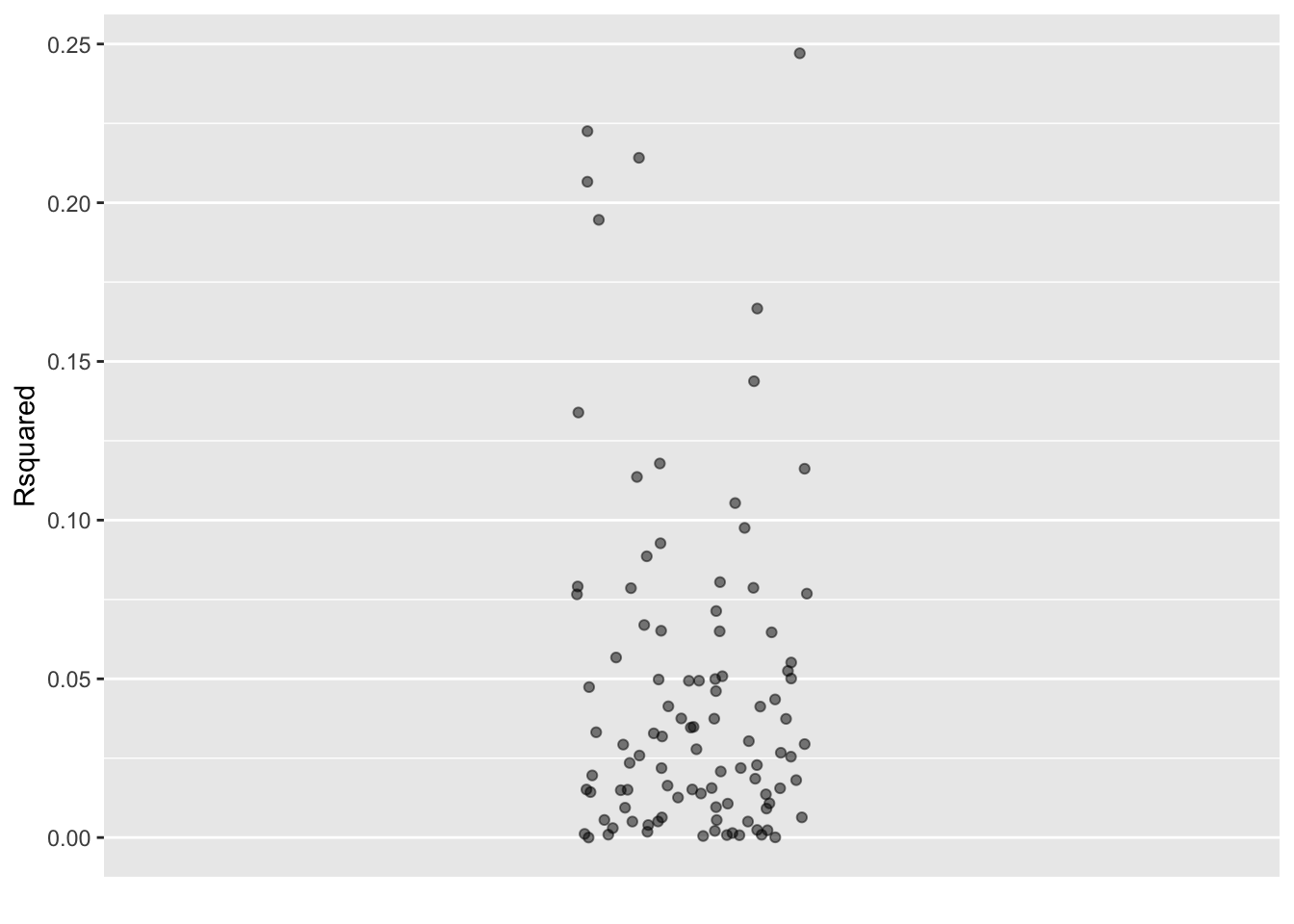
Data with a shuffled x variable.
If you count carefully you will find 101 dots in Figure 29.1. That’s because, when you weren’t looking I added the results when Data were not shuffled.
Can you tell which of the dots is from the non-shuffled data? You can’t, because the relationship in the non-shuffled data is not discernible in the fog of sampling variation created by the shuffles. Consequently, we “fail to reject the Null hypothesis.”
Noting our failure, let’s try again with a better study, one with much more data. That’s usually not a realistic possibility in an actual real-world-data study, but the simulation makes it easy.
Big_data <- Data <- Not_null_sim |> take_sample(n = 1000) Code
# No shuffling, the actual data
Actual <- Data |>  model_train(y ~ x) |>
  R2() |> select(n, k, Rsquared)
# 100 trials involving shuffling
Trials <- Data |>
  mutate(x = mosaic::shuffle(x)) |>
  model_train(y ~ x) |>
  R2() |> select(n, k, Rsquared) |>
  trials(100)
Together <- Actual |> bind_rows(Trials)
Together |>
  point_plot(Rsquared ~ 1)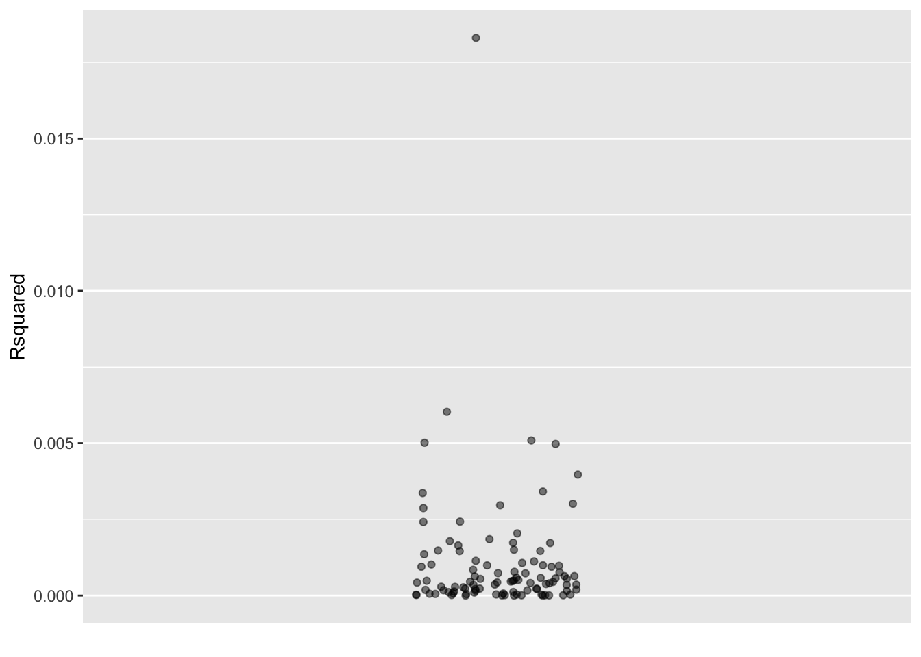
NHT and scientific method
Consider this mainstream definition of the scientific method:
“a method of procedure that has characterized natural science since the 17th century, consisting in systematic observation, measurement, and experiment, and the formulation, testing, and modification of hypotheses.” - Oxford Languages
It would be easy to conclude from this definition that “testing … of hypotheses” is central to science. However, the “hypotheses” involved in the scientific method are not the “Null hypothesis” that is implicated in NHT.
A famous example of a genuine scientific hypothesis is Newton’s law of gravitation from 1666. This hypothesis was tested in various ways: predictions of the orbits of the planets and moons around planets, laboratory detection of minute attractions in experimental apparatus, and so on. In the mid-1800s, it was observed that the movement of Mercury was not entirely in accord with Newton’s law. This is an example of scientific testing of a hypothesis; Newton’s law failed that test. In response, various theoretical modifications were offered, such as the presence of a hidden planet called Vulcan. These were ultimately unsuccessful. However, in 1915, Einstein published a modification of Newton’s gravitation called “the theory of general relativity.” This correctly accounts for the motion of Mercury. Additional evidence (such as the bending of starlight around the sun observed during the 1919 total eclipse) led to the acceptance of general relativity. The theory has continued to be tested, for example looking for the actual existence of “black holes” predicted by general relativity.
The Null hypothesis is different. The same Null hypothesis is used in diverse fields: biology, chemistry, economics, geology, clinical trials of drugs, and so on, more than can be named. This is why the Null is taught in statistics courses rather than as a principle of science. Nonetheless, the Null hypothesis plays important roles in the sociology and management of science. NHT is a standard operating procedure (SOP) that supports scientists and managers of scientific funding to examine results of preliminary work to form an opinion about whether a follow-up might be fruitful. The NHT SOP is also used by journal editors to screen submitted papers.
Standard operating procedures are methods, rules, or actions established for performing routine duties or in designated situations. SOPs are usually associated with organizations and bureaucratic operations such as hiring a new worker or responding to a report of broken equipment or a spilled chemical. SOPs are intended to routinize operations and help coordinate different components of the organization.
There are SOPs important to scientific work. For example, research with human subjects undergoes an “institutional review” SOP that ensures safety and that subjects are thoroughly informed about risk.
I think that “hypothesis testing,” is best seen as an SOP, a statistical procedure intended to inform decision-making by researchers, readers, and editors of scientific publications. For example, an individual researcher or research team needs to assess whether the data collected in an investigation is adequate to serve the intended purpose. A reader of the scientific literature needs a quick way to assess the validity of claims made in a report. A journal editor, needs a straightforward means to screen submitted manuscripts to check that the claims are supported by data and that the claims are novel to the journal’s field. The hypothesis testing SOP is designed to serve these needs. The words “adequate,” “quick,” and “straightforward” in the previous sentences correctly reflect the tone of hypothesis testing.
Science is often associated with ingenuity, invention, creativity, deep understanding, and the quest for new knowledge. Perhaps understandably, “SOP” rarely appears in reports of new scientific findings. Unfortunately, failing to see “hypothesis testing” as an SOP results in widespread misunderstanding and a bad habit of leaning on p-values and the misleading word “significance” to give support that cannot be provided by the logic behind NHT.
Exercises
EXERCISE: Count the dots from a shuffling trial that are bigger than the actual dot.
Enrichment Topics
Enrichment topic 29.1: Confidence level as a long-run frequency (DRAFT)
You will get your reward in heaven.
Enrichment topic 29.2: R2 and p for a categorical explanatory variable (DRAFT)
Show R2() and conf_intervals() for models with a single categorical variable.
- When there are two levels, the p-value on the coefficient is identical to the p-value on R2.
- When there are multiple levels, this is not true. There will, of course, be multiple coefficients, each with a p-value. The R2 collects together the explanatory umph of all the levels, but it also how many coefficients are used to achieve the result.
Enrichment topic 29.3: The “significance” level (DRAFT)
You may recall from Lesson ?sec-confidence-interval that part of constructing a confidence interval was to specify a confidence level . We have paid little attention to this simply because accepted practice is to set the confidence level at 0.95. Properly speaking, the intervals construct at this level are called “95% confidence intervals.”
You can, if you like, use a level other than 95% by setting the level = argument to conf_interval(). To illustrate, we will compute the confidence intervals at several different levels of the coefficients from the same model.
Confidence intervals on the same model, but at different confidence levels.
Model <-
  Not_null_sim |> take_sample(n = 1000) |>
  model_train(y ~ x)
Model |> conf_interval(level = 0.80) |> filter(term == "x")| term | .lwr | .coef | .upr |
|---|---|---|---|
| x | 0.0338541 | 0.0732575 | 0.1126609 |
Model |> conf_interval(level = 0.90) |> filter(term == "x")| term | .lwr | .coef | .upr |
|---|---|---|---|
| x | 0.0226703 | 0.0732575 | 0.1238447 |
Model |> conf_interval(level = 0.95) |> filter(term == "x")| term | .lwr | .coef | .upr |
|---|---|---|---|
| x | 0.0129619 | 0.0732575 | 0.133553 |
Model |> conf_interval(level = 0.99) |> filter(term == "x")| term | .lwr | .coef | .upr |
|---|---|---|---|
| x | -0.0060399 | 0.0732575 | 0.1525548 |
Model |> conf_interval(level = 1.00) |> filter(term == "x")| term | .lwr | .coef | .upr |
|---|---|---|---|
| x | -Inf | 0.0732575 | Inf |
You can see from the output from ?lst-confidence-levels that making the confidence level higher makes the confidence interval broader. You can also see that asking for “complete confidence” in the form of a confidence level of 100% leads to a complete lack of information: the confidence interval for level = 1.00 is infinitely broad.
You can, if you like, use a confidence level other than 95%. When such a confidence interval is used in a hypothesis test, statisticians use a different nomenclature that avoids the word “confidence.” Instead, they look at one minus the confidence level, calling this number the “significance level.” For instance, a hypothesis test conducted with a 95% confidence interval is said to be at the 0.05 level of significance. Referring to the output of ?lst-confidence-intervals, you can see that the hypothesis test at a 0.05 or higher level of significance concludes to “reject the Null hypothesis.” But a hypothesis test at the 0.01 significance level (that is, confidence level of 99%), “fails to reject the Null.”
It’s tempting to view confidence intervals with the eyes of a Bayesian, with the confidence level specifying how sure we want to be in a claim like this: “The true value of the coefficient has a probability of 95% of falling in the 95% confidence interval, and similarly for other confidence levels.” Such intervals can be calculated—in the Bayesian lingo they are called “credible intervals.” But Bayesian reasoning always involves a prior, and the point of hypothesis testing is to avoid any such thing.
Consequently, hypothesis
Enrichment topic 29.4: Analysis of variance (Draft)
Explain how it works and some of its uses.
Enrichment topic 29.5: Traditional tests (Draft)
Explain the context of each of the traditional tests and how it corresponds to the type of the explanatory variable(s).
What goes into a p-value: effect size divided by sample size.
Sampling distribution of p-values.
Hypothesis testing from a Bayesian perspective