noise_sim <- datasim_make(
  x <- rnorm(n),
  y <- rnorm(n)
)14 Simulation
Carl Wieman is a Nobel-prize-winning physicist and professor of education at Stanford University. Weiman writes, “For many years, I had two parallel research programs: one blasting atoms with lasers to see how they’d behave, and another studying how people learn.” Some of Wieman’s work on learning deals with the nature of “expertise.” He points out that experts have ways to monitor their own thinking and learning; they have a body of knowledge relevant to checking their own understanding.
This lesson presents you with tools to help you monitor your understanding of statistical methods. The monitoring strategy is based on simulation. In a simulation, you set up a hypothetical world where you get to specify the relationships between variables. The simulation machinery lets you automatically generate data collected in this hypothetical world. You can then apply statistical methods, such as regression modeling, to the simulated data. Then check the extent to which the results of the statistical methods, for instance model coefficients, agree with the hypothetical world that you created. If so, the statistical method is doing its job. If not, you have discovered limits to the statistical method, and you can explore how you might modify the method to give better agreement.
Like our data, the simulation involves a mixture of signal and noise. You implement the signal by setting precise mathematical rules for the relationships between your simulation variables. The noise comes in when we modify the mathematical rules to include measured amounts of noise.
Pure noise
We regard the residuals from a model as “noise” because they are entirely disconnected from the pattern defined by the tilde expression that directs the training of the model. There might be other patterns in the data—other explanatory variables, for instance—that could account for the residuals.
For simulation purposes, having an inexhaustible noise source guaranteed to be unexplainable by any pattern defined over any set of potential variables is helpful. We call this pure noise.
There is a mathematical mechanism that can produce pure noise, noise that is immune to explanation. Such mechanisms are called “random number generators.” R offers many random number generators with different properties, which we will discuss in Lesson sec-noise-models. In this Lesson, we will use the rnorm() random number generator just because rnorm() generates noise that looks generically like the residual that come from models. But in principle we could use others. We use datasim_make() to construct our data-generating simulations. Here is a simulation that makes two variables consisting of pure random noise.
Once a data-generating simulation has been constructed, we can draw a sample from it of whatever size n we like:
set.seed(153)
noise_sim |>take_sample(n = 5)| x | y |
|---|---|
| 2.819099 | -0.3191096 |
| -0.524167 | -1.3198173 |
| 1.194761 | -2.2864853 |
| -1.741019 | -0.7891444 |
| -0.449941 | -0.8128883 |
Although the numbers produced by the simulation are random, they are not entirely haphazard. Each variable is unconnected to the others, and each row is independent. Collectively, however, the random values have specific properties. The output above shows that the numbers tend to be in the range -2 to 2. In Figure fig-xy-random, you can see that the distribution of each variable is densest near zero and becomes less dense rapidly as the values go past 1 or -1. This is the so-called “normal” distribution, hence the name rnorm() for the random-number generator that creates such numbers.
Code
set.seed(106)
noise_sim |> datasim_run(n=5000) |>
  pivot_longer(c(x, y),
               names_to = "variable_name", values_to = "value") |>
  point_plot(value ~ variable_name, annot = "violin",
             point_ink = 0.1, size = 0)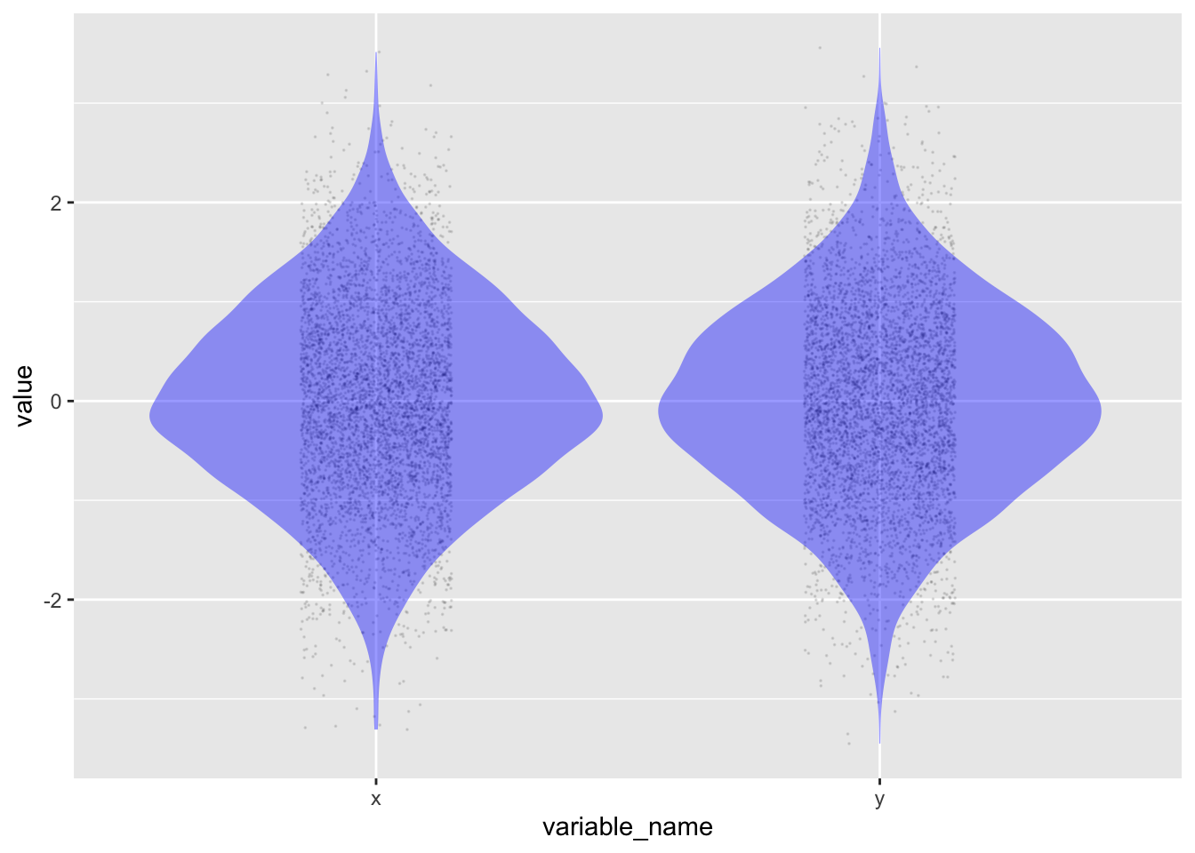
x and y variables from the simulation.
Another property of the numbers generated by rnorm(n) is that their mean is zero and their variance is one.
noise_sim |>take_sample(n=10000) |>
summarize(mean(x), mean(y), var(x), var(y))| mean(x) | mean(y) | var(x) | var(y) |
|---|---|---|---|
| 0.000382 | 0.00152 | 0.998 | 1 |
But they aren’t exactly what they ought to be!
Most people would likely agree that the means and variances in the above report are approximately zero and one, respectively, but are not precisely so.
This has to do with a subtle feature of random numbers. We used a sample size n = 10,000, but we might equally well have used a sample size 1. Would the mean of such a small sample be zero? If this were required, the number would hardly be random!
The mean of random numbers from rnorm(n) won’t be exactly zero (except, very rarely and at random!). But the mean will tend to get closer to zero the larger that n gets. To illustrate, here are the means and variances from a sample that’s 100 times larger: n = 1,000,000:
noise_sim |>take_sample(n=1000000) |>
summarize(mean(x), mean(y), var(x), var(y))| mean(x) | mean(y) | var(x) | var(y) |
|---|---|---|---|
| 0.00118 | 0.000586 | 1 | 0.999 |
The means and variances can drift far from their theoretical values for small samples. For instance:
noise_sim |>take_sample(n=10) |>
summarize(mean(x), mean(y), var(x), var(y))| mean(x) | mean(y) | var(x) | var(y) |
|---|---|---|---|
| 0.342 | -0.155 | 0.424 | 0.776 |
Recall the claim made earlier in this Lesson that rnorm() generates a new batch of random numbers every time, unrelated to previous or future batches. In such a case, the model y ~ x will, in principle, have an x-coefficient of zero. R2 will also be zero, as will the model values. That is, x tells us nothing about y. Figure fig-noise_sim verifies the claim with an annotated point plot:
Code
noise_sim |>take_sample(n=10000) |>
  point_plot(y ~ x, annot = "model",
             point_ink = 0.1, model_ink = 1, size=0.1) |>
  gf_theme(aspect.ratio = 1)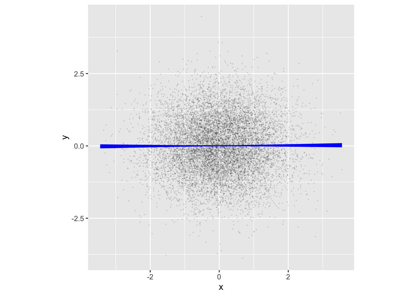
noise_sim. The round cloud is symptomatic of a lack of relationship between the x and y values. The model values are effectively zero; x has nothing to say about y.
Simulations with a signal
The model values in Figure fig-noise_sim are effectively zero: there is no signal in the noise_sim. If we want a signal between variables in a simulation, we need to state the data-generating rule so that there is a relationship between x and y. For example:
signal_sim <- datasim_make(
  x <- rnorm(n),
  y <- 3.2 * x + rnorm(n)
)
Code
signal_sim |>take_sample(n=10000) |>
  point_plot(y ~ x, annot = "model",
             model_ink = 1, point_ink = 0.1, size=0.1)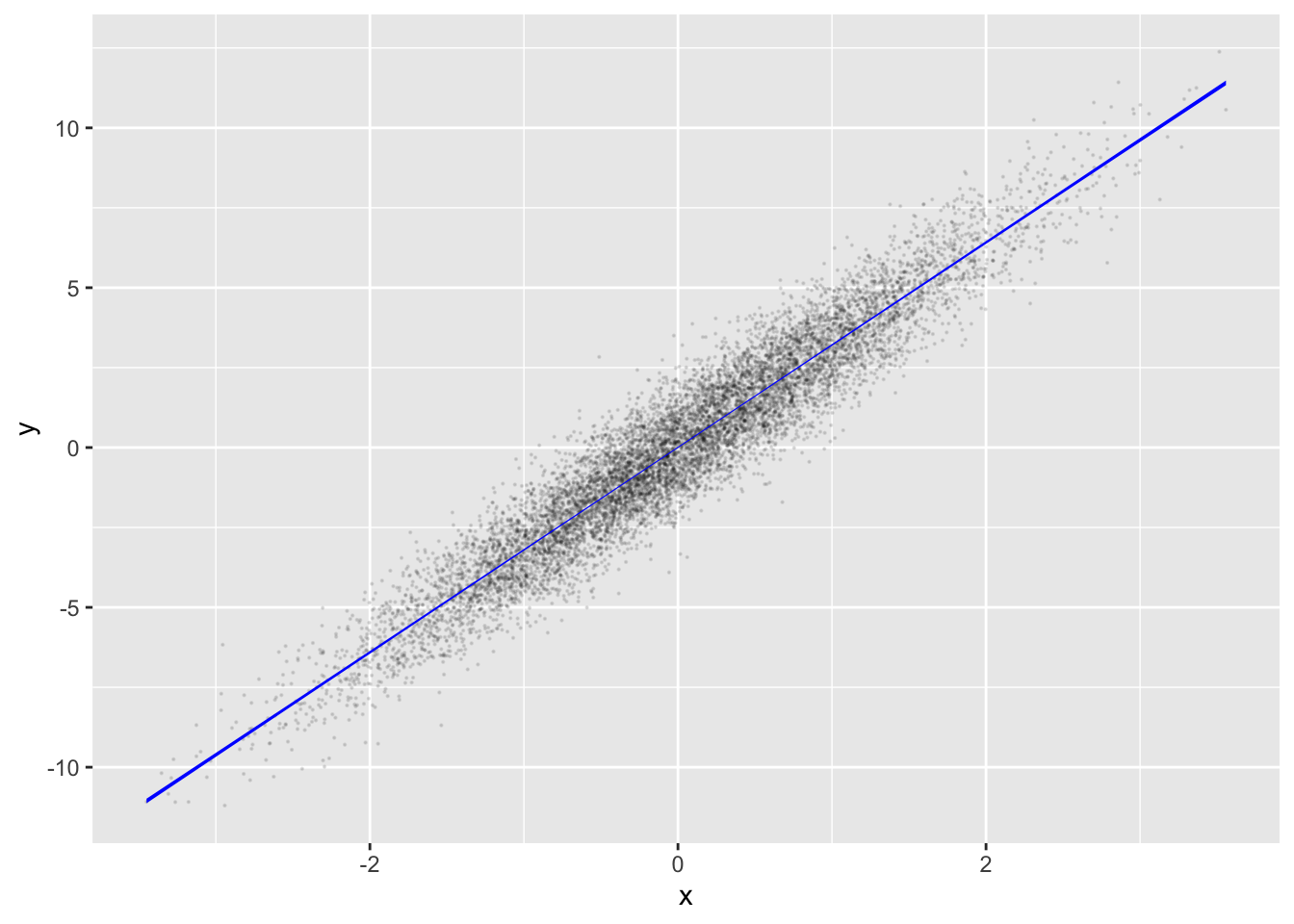
signal_sim where the y values are defined to be y <- 3.2 * x + rnorm(n). The cloud is elliptical and has a slant.
Example: Heritability of height
Simulations can be set up to implement a hypothesis about how the world works. The hypothesis might or might not be on target. It’s not even necessary that the hypothesis be completely realistic. Still, data from the simulation can be compared to field or experimental data.
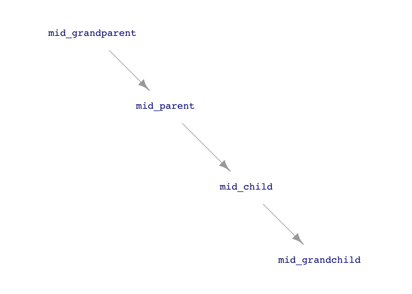
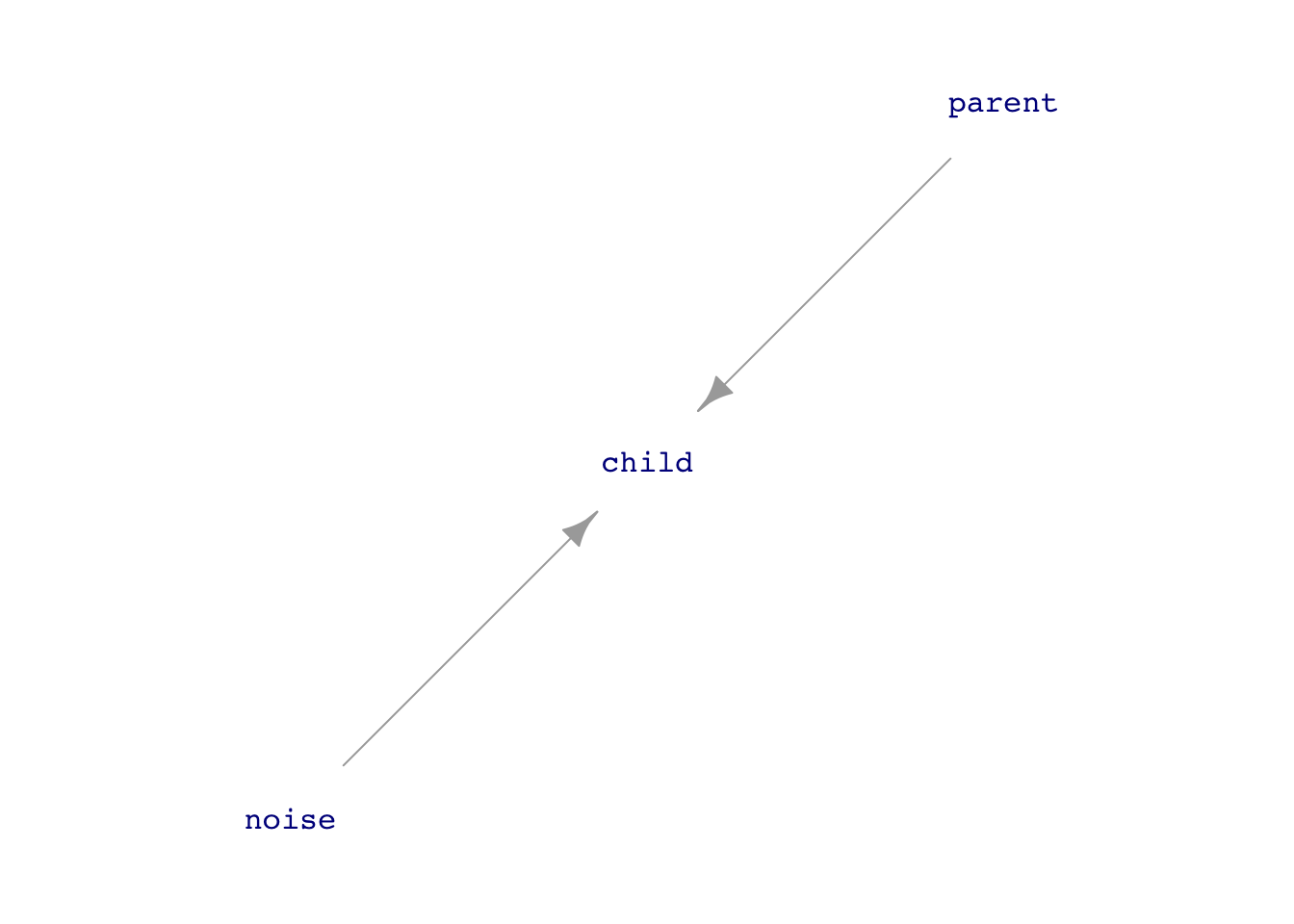
Consider the following simulation in which each row of data gives the heights of several generations of a family. The simulation will be a gross simplification, as is often the case when starting to theorize. There will be a single hypothetical “mid-parent,” who reflects the average height of a real-world mother and father. The children—“mid-children”—will have a height mid-way between real-world daughters and sons.
height_sim <- datasim_make(
  mid_grandparent <- 66.7 + 2 * rnorm(n),
  mid_parent <- 17.81 + 0.733 * mid_grandparent +  0.99 * rnorm(n),
  mid_child <- 17.81 + 0.733 * mid_parent + 0.99 * rnorm(n),
  mid_grandchild <- 17.81 + 0.733 * mid_child + 0.99 * rnorm(n)
)
Note that the formulas for the heights of the mid-parents, mid-children, and mid-grandchildren are similar. The simulation imagines that the heritability of height from parents is the same in every generation. However, the simulation has to start from some “first” generation. We use the grandparents for this.
We can sample five generations of simulated heights easily:
sim_data <- height_sim |>take_sample(n=100000)The simulation results compare well with the authentic Galton data:
Galton2 <- Galton |> mutate(mid_parent = (mother + father)/2)
Galton2 |> summarize(mean(mid_parent), var(mid_parent))| mean(mid_parent) | var(mid_parent) |
|---|---|
| 66.65863 | 3.066038 |
sim_data |> summarize(mean(mid_parent), var(mid_parent))| mean(mid_parent) | var(mid_parent) |
|---|---|
| 66.70651 | 3.098433 |
The mean and variance of the mid-parent from the simulation are close matches to those from Galton. Similarly, the model coefficients agree, with the intercept from the simulation data including one-half of the Galton coefficient on sexM to reflect the mid-child being halfway between F and M.
Mod_galton <- Galton2 |>
  model_train(height ~ mid_parent + sex)
Mod_sim    <- sim_data |>
  model_train(mid_child ~ mid_parent)
Mod_galton |> conf_interval()| term | .lwr | .coef | .upr |
|---|---|---|---|
| (Intercept) | 9.8042633 | 15.2013993 | 20.5985354 |
| mid_parent | 0.6520547 | 0.7328702 | 0.8136858 |
| sexM | 4.9449933 | 5.2280332 | 5.5110730 |
Mod_sim |> conf_interval()| term | .lwr | .coef | .upr |
|---|---|---|---|
| (Intercept) | 17.8402226 | 18.0725882 | 18.3049537 |
| mid_parent | 0.7257281 | 0.7292103 | 0.7326925 |
Mod_galton |> R2()| n | k | Rsquared | F | adjR2 | p | df.num | df.denom |
|---|---|---|---|---|---|---|---|
| 898 | 2 | 0.638211 | 789.4087 | 0.6374025 | 0 | 2 | 895 |
Mod_sim |> R2()| n | k | Rsquared | F | adjR2 | p | df.num | df.denom |
|---|---|---|---|---|---|---|---|
| 1e+05 | 1 | 0.6275154 | 168464.1 | 0.6275117 | 0 | 1 | 99998 |
Each successive generation relates to its parents similarly; for instance, the mid-child has children (the mid-grandchild) showing the same relationship.
sim_data |> model_train(mid_grandchild ~ mid_child) |> conf_interval()| term | .lwr | .coef | .upr |
|---|---|---|---|
| (Intercept) | 17.4321058 | 17.6846047 | 17.9371036 |
| mid_child | 0.7310966 | 0.7348802 | 0.7386638 |
… and all generations have about the same mean height:
sim_data |>
summarize(mean(mid_parent), mean(mid_child), mean(mid_grandchild))| mean(mid_parent) | mean(mid_child) | mean(mid_grandchild) |
|---|---|---|
| 66.70651 | 66.71566 | 66.71262 |
However, the simulated variability decreases from generation to generation. That’s unexpected, given that each generation relates to its parents similarly.
sim_data |>
summarize(var(mid_parent), var(mid_child), var(mid_grandchild))| var(mid_parent) | var(mid_child) | var(mid_grandchild) |
|---|---|---|
| 3.098433 | 2.625568 | 2.396332 |
To use Galton’s language, this is “regression to mediocrity,” with each generation being closer to the mean height than the parent generation.
Note
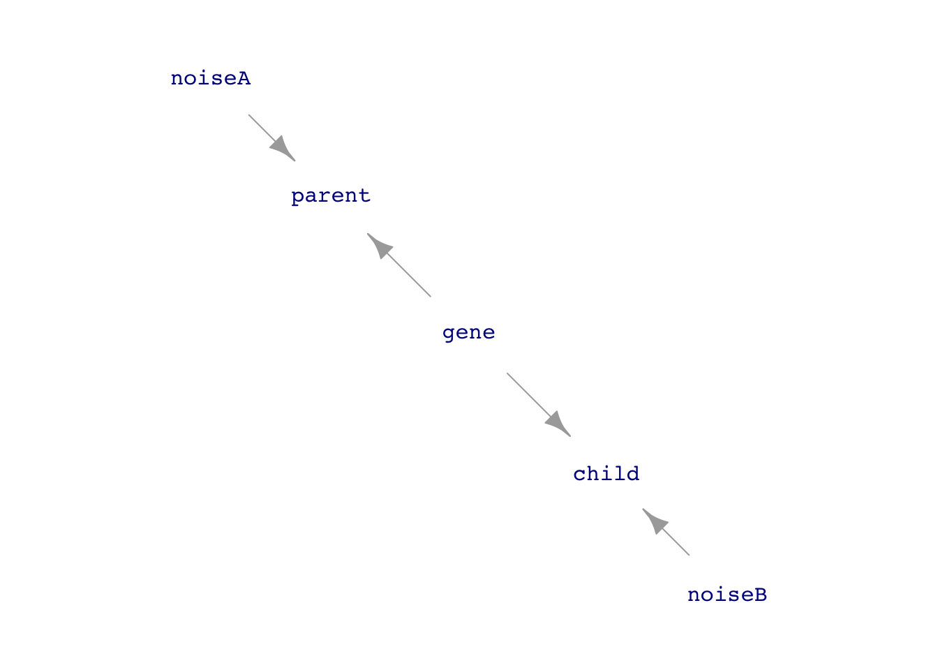
FYI … Phenotype vs genotype
Modern genetics distinguishes between the “phenotype” of a trait and the “genotype” that is the mechanism of heritability. The phenotype is not directly inherited; it reflects outside influences combined with the genotype. The above simulation reflects an early theory of inheritance based on “phenotype.” (See Figure fig-genotype-phenotype.) However, in part due to data like Galton’s, the phenotype model has been rejected in favor of genotypic inheritance.
Activity 14.1
A few problems involving measuring the relative widths of the violins at different values of the y variable.
Activity 14.2
- Make a simulated
xlike this:
This_sim <- datasim_make(
  x <- rnorm(n),
  y <- x + rnorm(n)
)
Dat <- This_sim |>take_sample(n = 1000)
a. In `Dat`, what is the variance of `x`? That is, what is the variance of the values generated by `rnorm(n)`
b. What is the variance of `y`?
c. Change the rule for `y` to `y <- rnorm(n) + rnorm(n) + rnorm(n)`. What will be the variance of the sum of three sequences generated from this new rule for `y`?If your conclusions are uncertain, make the sample size much bigger, say sample(n = 1000000). That should clarify the arithmetic?
- Use a new rule
y = rnorm(n) + 3 * rnorm(n). What is the variance ofyfrom this rule?
Activity 14.3
When modeling the simulated data using the specification child ~ mom + dad, the coefficients were consistent with the mechanism used in the simulation.
Explain in detail what aspect of the simulation corresponds to the coefficient found when modeling the simulated data.
As you explained in (a), the specification
child ~ mom + dadgives a good match to the coefficients from modeling the simulated data, and makes intuitive sense. However, the specificationdad ~ child + momdoes not accord with what we know about biology. Fit the specificationdad ~ child + momto simulated data and explain what about the coefficients contradicts the intuitive notion that the mother’s height is not a causal influence on the father’s height.
Activity 14.4
INTRODUCE trials()
BUILD MODELS and show the coefficients are close to zero, but not exactly. R2 is close to zero, but not exactly. Run many trials and ask what the variance of the trial-to-trial means is. How does it depend on \(n\)?
Activity 14.5
Accumulating variation
set.seed(103)
Large <-take_sample(sim_01, n=10000)
Lesson sec-measuring-variation introduced the standard way to measure variation in a single variable: the variance or its square root, the standard deviation. For instance, we can measure the variation in the variables from the Large sample using sd() and var():
Large |>
summarize(sx = sd(x), sy = sd(y), vx = var(x), vy = var(y))| sx | sy | vx | vy |
|---|---|---|---|
| 0.9830639 | 1.779003 | 0.9664146 | 3.164851 |
According to the standard deviation, the size of the x variation is about 1. The size of the y variation is about 1.8.
Look again at the formulas that compose sim_01:
print(sim_01)Simulation object
------------
[1] x <- rnorm(n)
[2] y <- 1.5 * x + 4 + rnorm(n)The formula for x shows that x is endogenous, its values coming from a random number generator, exo(), which, unless otherwise specified, generates noise of size 1.
As for y, the formula includes two sources of variation:
- The part of
ydetermined byx, that is \(y = \mathbf{1.5 x} + \color{gray}{4 + \text{exo()}}\) - The noise added directly into
y, that is \(y = \color{gray}{\mathbf{1.5 x} + 4} + \color{black}{\mathbf{exo(\,)}}\)
The 4 in the formula does not add any variation to y; it is just a number.
We already know that exo() generates random noise of size 1. So the amount of variation contributed by the + exo() term in the DAG formula is 1. The remaining variation is contributed by 1.5 * x. The variation in x is 1 (coming from the exo() in the formula for x). A reasonable guess is that 1.5 * x will have 1.5 times the variation in x. So, the variation contributed by the 1.5 * x component is 1.5. The overall variation in y is the sum of the variations contributed by the individual components. This suggests that the variation in y should be \[\underbrace{1}_\text{from exo()} + \underbrace{1.5}_\text{from 1.5 x} = \underbrace{2.5}_\text{overall variation in y}.\] Simple addition! Unfortunately, the result is wrong. In the previous summary of the Large, we measured the overall variation in y as about 1.8.
The variance will give a better accounting than the standard deviation. Recall that exo() generates variation whose standard deviation is 1, so the variance from exo() is \(1^2 = 1\). Since x comes entirely from exo(), the variance of x is 1. So is the variance of the exo() component of y.
Turn to the 1.5 * x component of y. Since variances involve squares, the variance of 1.5 * x works out to be \(1.5^2\, \text{var(}\mathit{x}\text{)} = 2.25\). Adding up the variances from the two components of y gives
\[\text{var(}\mathit{y}\text{)} = \underbrace{2.25}_\text{from 1.5 exo()} + \underbrace{1}_\text{from exo()} = 3.25\]
This result that the variance of y is 3.25 closely matches what we found in summarizing the y data generated by the DAG.
The lesson here: When adding two sources of variation, the variances of the individual sources add to form the overall variance of the sum. Just like \(A^2 + B^2 = C^2\) in the Pythagorean Theorem.
Activity 14.6
sec-pure-noise claims that two variables made by separate calls to rnorm() will not have any link with one another. Let’s test this:
test_sim <- datasim_make(
  x <- rnorm(n),
  y <- rnorm(n)
)
Samp <- test_sim |>take_sample(n = 100)
Train the model y ~ x on the data in Samp.
In principle, what should the
xcoefficient be fory ~ xwhen there is no connection? Is that what you find from your trained model?In principle, what should the R2 be for
y ~ xwhen there is no connection? Is that what you find from your trained model?Make the sample 100 times larger, that is
n = 10000. Does your coefficient (from (1)) or your R2 (from (2)) get closer to their ideal values?Make the sample another 100 times larger, that is
n=1000000. Does your coefficient (from (1)) or your R2 (from (2)) get closer to their ideal values?