The kind of thing represented by a row of a data frame. Properly, each and every row is the same kind of thing. That is, there is only one unit of observation for each data frame, no matter how many rows there are.
A value for each specimen of the same kind of thing, e.g. temperature or age.
The name “variable” is a reminder that the values in a column of a data frame can differ from one another. That is, they vary from specimen to specimen. For instance, in a data frame where the unit of observation is a person, the variable age will have values that (typically) are not all the same.
A variable for which the values are numerical, often with physical units. Properly, all the values in a quantitative variable are recorded in the same physical units, e.g. kilometers. Don’t mix, e.g. kilometers and miles in the same variable.
The complete list of the possible values recorded in a categorical variable. Example: a categorical variable whose values are days of the week might have levels Sunday, Monday, Tuesday, Wednesday, Thursday, Friday, Saturday.
Ideally, a complete enumeration of all of the specimens in existence in the world. A data frame containing a census comprehends every possible one of the unit of observation.
In Lessons, we use “table” to refer to an arrangement of information directed at the human reader. As such, tables often violate the basic principles of tidy data frames. For instance, tables may contain summaries of other rows, for instance the “total” of preceeding entries.
The documentation for a data frame that describes what is the unit of observation as well as what each of the variables represents, its physical units (if any). For categorical variables, the documentation (ideally) explains what each level means, particularly when they are abbreviations.
A computer/web application that provides services for accessing R. For example, RStudio provides an editor for writing documents that can use R for internal computation.
(computing) The kind of thing that carries out a computation, that is, transforms one or more inputs into an output. Example: nrow() takes a data frame as input and gives as output the number of rows in that data frame.
(computing) Each data frame in a package has its own name, by which you can refer to the data frame itself.
package::name
(computing) Two or more packages may use the same name to refer to distinct data frames, in much the same way as the name George can belong to more than one person. With people, we can distinguish between those different people by using their family name as well as their first name, e.g. George Washington. In R, the analogous syntax consists of the package name followed by two colons which are in turn followed by the data frame name. This avoids potential confusion by telling R where to look for the data frame. Example: mosaicData::Galton directs R to the data frame named Galton from the mosaicData package.
LSTbook
(computing) The name of the package that contains many of the data frames and functions most used in Lessons.
library(LSTbook)
(computing) A command that directs R to “load” the LSTbook data frame so that you can refer to its data frames and functions without needing the double-colon syntax.
(computing) A syntax for providing an input to a function. For instance, here’s how to find the number of rows in Births2022: give the Births2022 data frame as input to the nrow() function:
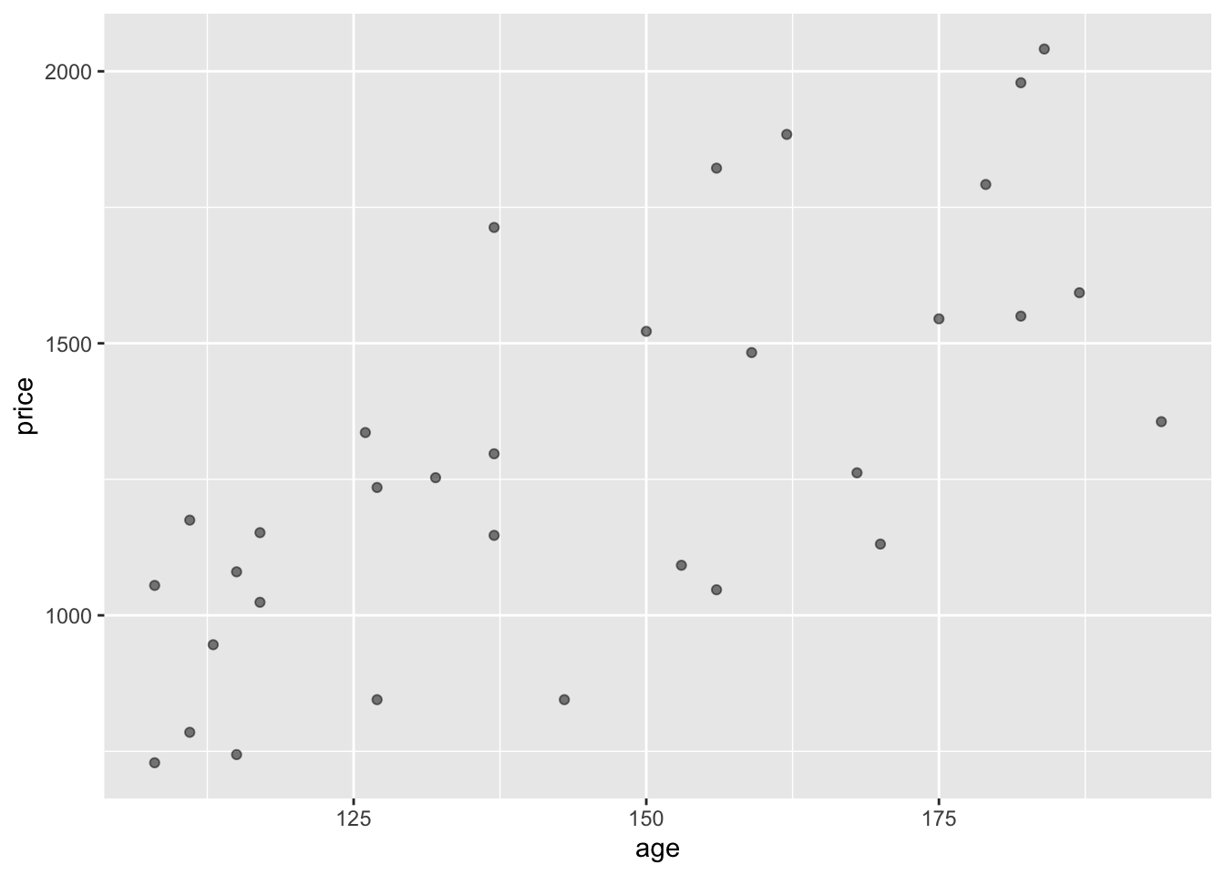
The spatial region encompassed by a graphic and given meaning by a cartesian coordinate system. Each of the axes in the coordinate system refers to a single variable. In a point plot, each dot is situated within the graphics frame.
Clock_auction |>point_plot(price ~ age)
Figure 30.1: A point plot consists of dots placed inside a graphics frame.
y axis
The vertical axis of a graphics frame.
x axis
The horizontal axis of a graphics frame.
“Mapped to”
Shorthand to describe which variable is represented by each graphics axis. In Figure 30.1, the variable price is mapped to y, which the variable age is mapped to x.
A variable selected by the modeler to be a source of explanation for the response variable. There can be more than one explanatory variable in a model.
(computing) The syntax used to indicate which variable is to be the response variable and which other variables are to be the explanatory variables. In Figure 30.1, the tilde expression is price ~ age. (The squiggly character in the middle, , is called a “tilde.”)
point_plot()
(computing) The function from the LSTbook package for making annotated point plots. Two inputs are required, a data frame and a tilde expression. The data frame is piped into point_plot(), while the tilde expression is placed inside the parentheses.
“mapped to color”
A tilde expression used in point_plot() can have more than one explanatory variable. If there are two (or more), the second explanatory variable is represented by color.
When the tilde expression used in point_plot() has three explanatory variables, the second is mapped to color while the third is mapped to facet.
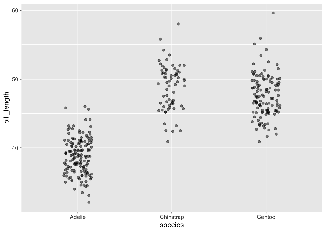
Penguins |>point_plot(bill_length ~ mass + sex + species)
Figure 30.2: A point plot of the Penguins data frame with three explanatory variables: mass is mapped to x, sex mapped to color, and species is mapped to facet. The response variable is bill_length.
A graphical technique for graphics frames in which a categorical variable is mapped to the x- or y-axis. Rather than all the specimens with the same level of the variable being placed at the same point along that axis, the specimens are randomly spread out a little around that point. This makes it easier to see as distinct dots that would otherwise be overlapping. See Figure 30.3(b).
Each dot in a point plot corresponds to an individual specimen from the data frame that’s being plotted. A graphical annotation is another kind of mark that represents the specimens collectively rather than as individuals.
For categorical variables (such as species in Figure 30.3) the different levels of the variable are discrete. There are no values for species that are in-between the discrete levels. On a point plot, there is empty space between any two levels of the species variable. For example, there’s no such thing as the species being half Adelie and half Gentoo.
In point_plot(), any variables that are mapped to color or mapped to facet are displayed as discrete variables, even if the variable itself is quantitative. This is done to make interpretation of the graphic easier. Later lessons will introduce the non-graphical techniques used to treat quantitative explanatory variables without converting them to discrete levels.
This Lesson continues with graphical presentations of data, focusing on graphical annotations that display the “shape” of variation. In contrast, Lesson 9 presents quantitative measures of variation.
The graphical presentations focus on the variation in the response variable, that is, the variable mapped to y. In a point plot, the variation in the response variable corresponds to the spread of dots along the y-axis.
In a point plot, dots that are neighbors along the y axis may be close together or not. The closeness of dots in a neighborhood is called the “density” in that neighborhood. In a high-density neighborhood, dots tend to be close together. Conversely, in a low-density neighborhood, dots are spaced farther apart. Naturally, different neighborhoods can have different densities.
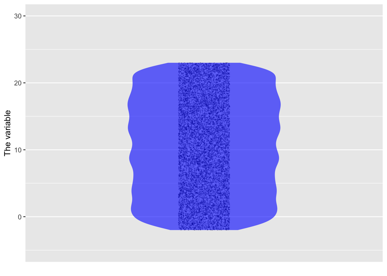
The pattern of density at different places the y axis. There are all sorts of possible patterns, but often we describe the distribution in words by referring to any of a handful of named patterns: “uniform,” “normal,” “long-tailed,” “skew.”
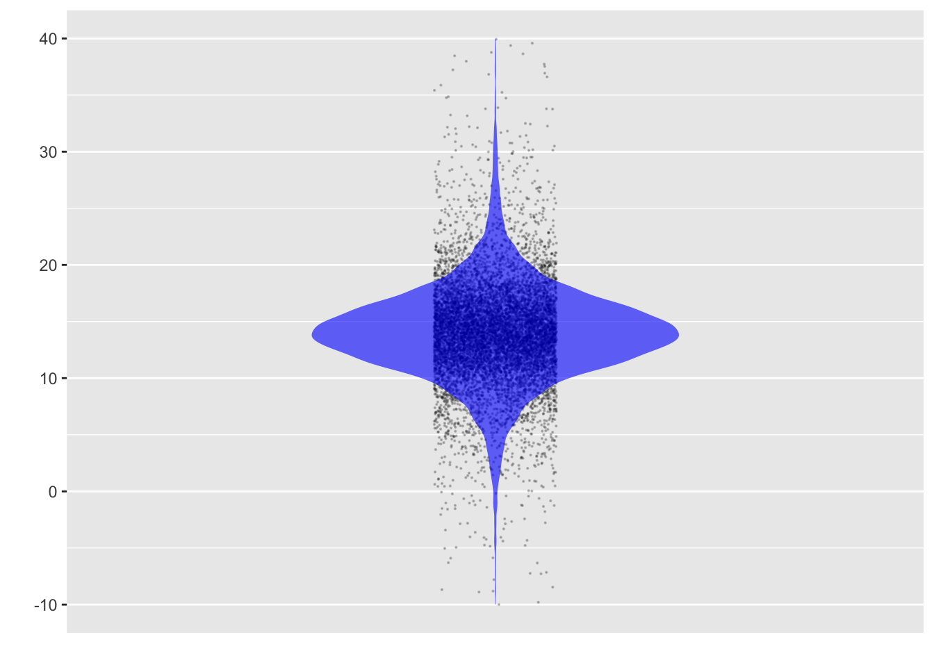
A distribution pattern where the density is at a peak at one value of y, falling off gradually and symmetrically with distance from that peak. The fall off is slow near the peak, faster somewhat further away from the peak but gradually approaching zero far from the peak. The normal distribution has a specific quantitative form for this fall off, often described as a “bell” shaped. Remarkably, the normal distribution is encountered frequently in practice, which explains why the word “normal” is used to name the pattern.
The y value that is in the middle of the distribution of dots. For a uniform distribution, the center is at the mid-point in y of the interval where the density is non-zero. For a normal distribution, the center is the y value where the peak density occurs.
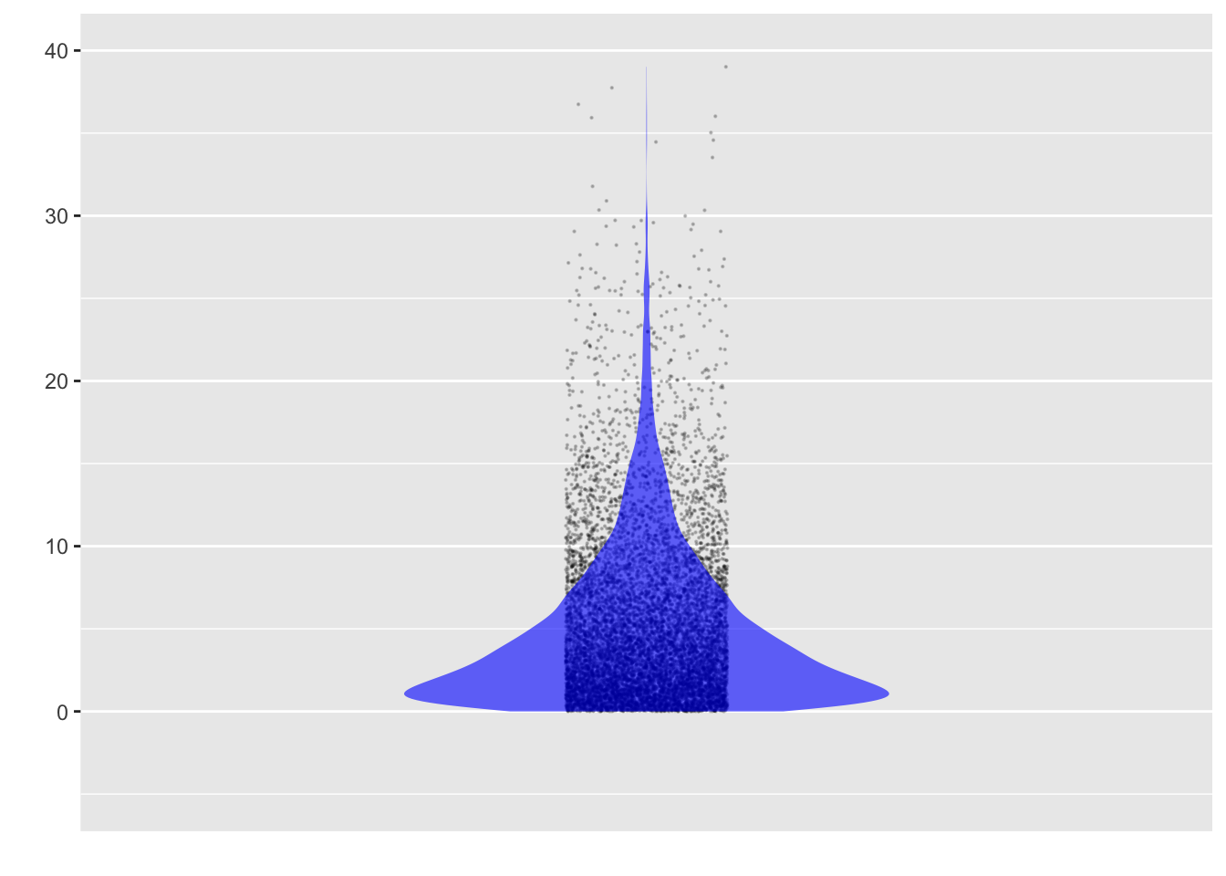
A distribution pattern where values far from the peak are considerably more common than seen in the “normal” distribution. Being precise about the meaning of “more common” depends on a numerical description of distributions, which we will talk about in later Lessons. In Figure 30.4, the long tail is indicated by “spikes” at either end of the distribution, spikes that are much sharper than for the “normal” distribution.
A distribution pattern where one tail is long but the other is not.
(a) Uniform
(b) Normal
(c) Long tailed
(d) Skew
Figure 30.4: Various distribution shapes
Lesson 4: Annotating point plots with a model
The “violin,” introduced in Lesson 3 is one form of annotation for a point plot. This lesson concerns another, completely different form of annotation on a point plot that highlights the relationship between two or more variables.
A representation of the pattern of relationship between a response variable and a single explanatory variable. We will focus on simple models for this section of the glossary.
A representation of the pattern of relationship between a response variable and one or more explanatory variables. Lesson 10 will cover such models in more detail.
Phrases signifying that the statement is about the dots collectively rather than individually. For example, in Figure 30.5(a), the individual dots are spread over a wide vertical region. There are females whose bills are longer than most males, and males whose bills are shorter than most females. So, refering to individual specimens, it’s not correct to say that females have shorter bills than males. But, to judge from the figure and the model annotations, it is correct to say that females tend to have shorter bills than males. The “tend to have” indicates that we are refering to females collectively, versus males collectively. The center of the female distribution of bill lengths is lower than the center of the male distribution of bill lengths.
To make an analogy to the world of team sports … It’s common to hear that Team A is better than Team B. If we were referring to the performance of individual players, it may well be that some Team-A players are worse than some Team-B players. We would use the statistical phrase “tend to be” if we wanted to indicate the collective properties of the whole team.
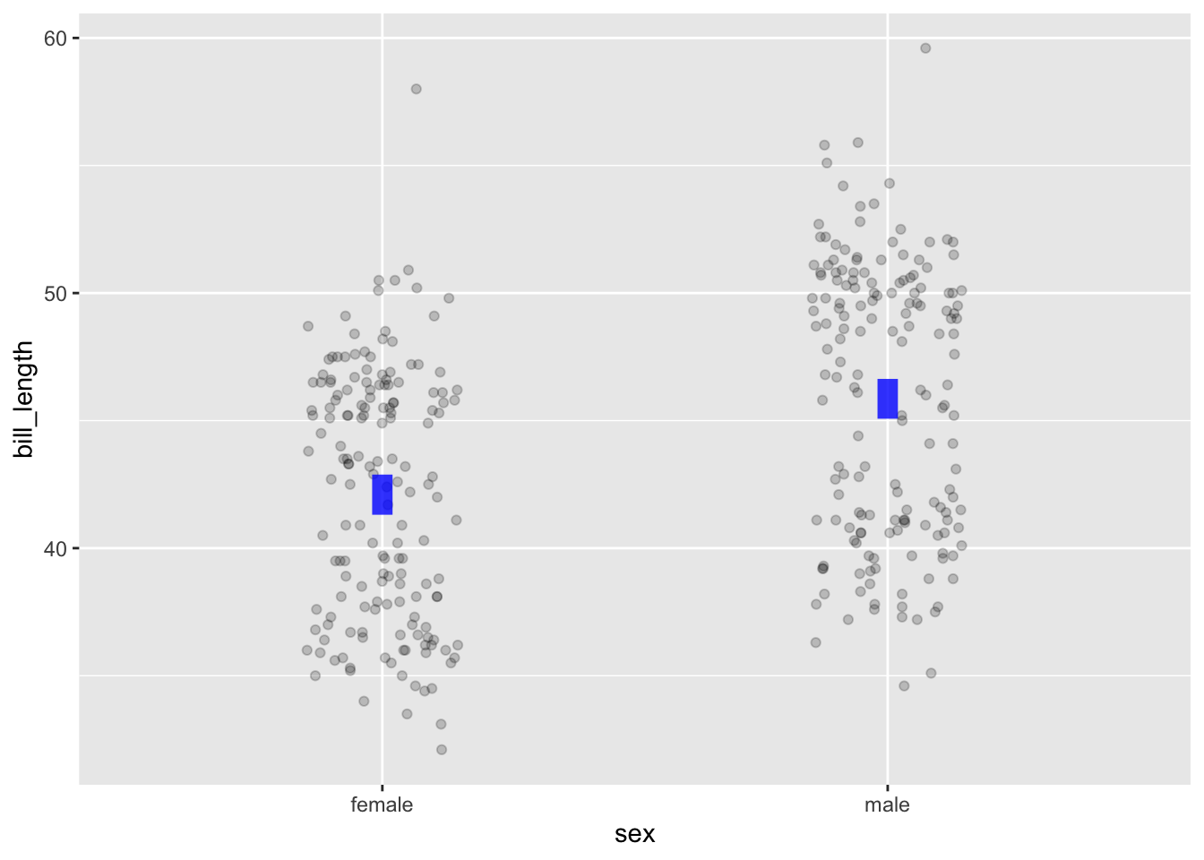
A type of model annotation appropriate when an explanatory variable is categorical. (But, remember, the response variable is always quantitative.) Typically there are two or more levels for a categorical variable, each level will have its own interval annotation. The relationship between the two variables is indicated by the vertical offset among the levels.
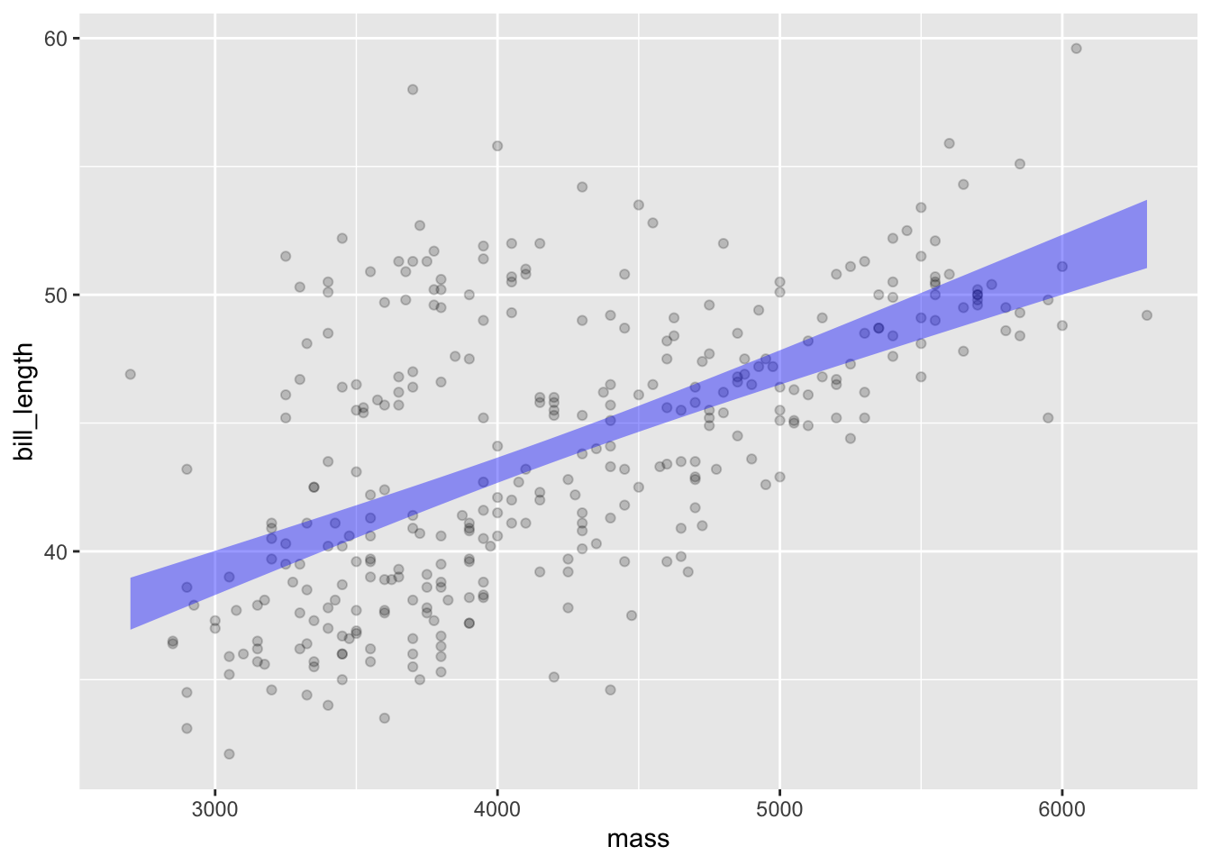
A type of model annotation to depict the relationship between two quantitative variables. The relationship is indicated by the slope of the band. A slope that is zero (that is, a horizontal band) suggests that the two variables are independent.
Figure 30.5: There are two situations for a model of the relationship between two variables. If the explanatory variable is categorical (Panel (a)), each level of that variable is annotated with an interval that designates a part of the y axis. If the explanatory variable is quantitative (Panel (b)), there is a continuous band.
In Panel (a), the vertical offset between the two intervals indicates a relationship between bill_length and sex. (In everyday language, this is simply that males tend to have longer bills than females.) In Panel (b), the non-zero slope indicates the relationship. Here, the slope is positive, indicating that penguins with larger body mass tend to have longer bills.
Although there are infinitely different ways to wrangle data, the most common ways can be implemented using a handful of basic operations applied in sequence: the “big 5” are filter, mutate, select, arrange, summarize. In some cases, more intricate/advanced operations are also needed: join and pivot, for example. This lesson focusses on the “big 5.”
A basic wrangling operation where the rows in the new data frame are re-ordered from the original according to one or more of the variables. For instance, the rows might be placed in numerical order based on a quantitative variable, or alphabetical order based on a categorical variable.
A wrangling operation which combines two data frames into a single data frame. Examples of joins are given in Lesson 7. Experience shows that it takes considerable practice to understand how joins work, in contrast to the basic wrangling operations filter, mutate, …, summarize, which correspond to basic clerical actions.
(computing) Each of the wrangling operations is applied using a corresponding R function. Those functions take a data frame as input and also are given additional arguments to specify the “details” of the operation, for instance what variable to use for arranging the rows.
(computing) Another word for the inputs to a function. Wrangling functions always take a data frame as input, but they need additional inputs to specify the particulars of the desired operation. In Lessons, we use a “pipeline” notation where the primary input—a data frame for wrangling functions—is sent via a pipe to the function. The additional arguments to the function are placed in the parentheses that follow the function name. Example: Penguins |> arrange(species).
(computing) A style suited to situations where a function has more than one argument and it is desired to be clear which argument we are referring to. For example, in Penguins |> point_plot(bill_length ~ species, annot = "model"), the expression annot = "model" means that the input named annot is to be given the value "model".
Lesson 6: Computing
This lesson is a review of the structure of the computing commands that have been encountered in the first five Lessons and which will be used in all later Lessons.
The style in which Lessons write commands in which the output of one function is sent to another for further processing. Example: Penguins |> arrange(bill_length) |> head(10) which has the effect of collecting into a new data frame the 10 specimens from Penguins that have the shortest bill lengths.
(computing) Giving a name to the output of a computing command so that that output can easily be used later on. A more widely used word for this is “assignment,” but we avoid that in Lessons because the everyday word has other meanings (e.g. a bit of required work).
(computing) The punctuation <- used to direct the computer to store an output under a specified name. Example: Shortest <- Penguins |> arrange(bill_length) |> head(10) will store a data frame with the ten shortest-billed specimens from Penguins under the name Shortest. Once stored, that data frame can be referred to by name in the same way as any other data frame.
Note about storage. In Lessons, we don’t need storage very often because the pipeline style allows us to send the output of a computing command directly as an input to another function, without having to name it. But, occasionally, we need to use that output for more than one function, in which case storage/naming is useful.
(computing) As you know, a data frame consists of one or more variables, each of which has a name. In Lessons, variable names will be used only in the arguments to functions. You will never use a variable name on its own. Example: SAT |> filter(frac > 50) where the variable name frac is used within the parentheses following the function name filter().
(computing) A meaningful fragment of a computing command. For instance, in SAT |> filter(frac > 50), one expression is frac > 50. filter(frac > 50) is also an expression. Commands are contructed out of expressions; think of them as the phrases in a sentence. Example: “above and beyond” is an expression but not a complete sentence like “She went above and beyond her obligations.”
(computing) Often, we need to use expressions that refer literally to a set of characters that is not the name of a function or data frame or variable name. Example: Penguins |> point_plot(bill_length ~ species, annot = "model"). The quotation marks in "model" indicate that it is to be used literally, and not to refer to something such as a variable name. Computing professionals use the phrase “character string” to refer to such quoted things as "model".
A set of well-organized data frames, each with its own unit of observation. “Well-organized” is not a technical term. An important part of good organization is that each of the data frames has one or more columns that can be used to look up values in another of the data frames or more than one.
(computing) The generic name for wangling operations where values from one data frame are inserted into appropriate rows of another data frame. (The Lesson shows a frequently type of join is called left_join().) The join operations are central to database use, since they enable information to be brought together from multiple data frames.
A numerical measure of the amount of variation in a quantitative variable.
The units of variance are important. Suppose the values in a variable have units of dollars. The variance has units of dollars-squared. If a variable is recorded in units of meters, the variance has units of square-meters. Around 1800, there were three different popular measures of variation. Counter-intuitively (but usefully), the winner involved the square units.
Numerically, simply the square root of the variance. In LST, we prefer to use the variance itself: why introduce extra square roots? The name “standard deviation” is strange and off-putting. The “standard” refers to the measure being widely accepted. “Deviation” is an old and obsolute term for what is now called “variation.”
At the heart of variance is averaging the squared differences between every pair of specimens in a variable. For instance, consider this data frame:
City
districts
New York
5
Boston
3
New Haven
1
Hartford
2
As you can see, the districts variable shows variation. Let’s enumerate all the pairwise square differences in the districts variable: there are six of them. (5-3)2, (3-1)2, (1-2)2, (5-1)2, (5-2)^2, and (3-2)2. Averaging these six pairwise square differences and dividing by two gives the variance. : There are much, much more efficient ways of calculating the variance. But thinking about variance in terms of pairwise differences is perhaps the easiest way to understand what variance is about.
Lesson 9: Accounting for variation
The word “account” has several related meanings. These definitions are drawn from the Oxford Languages dictionaries.
To “account for something” means “to be the explanation or cause of something.” [Oxford Languages]
An “account of something” is a story, a description, or an explanation, as in the Biblical account of the creation of the world.
To “take account of something” means “to consider particular facts, circumstances, etc. when making a decision about something.”
Synonyms for “account” include “description,”report,” “version,” “story,” “statement,” “explanation,” “interpretation,” “sketch,” and “portrayal.” “Accountants” and their “account books” keep track of where money comes from and goes to.
These various nuances of meaning, from a simple arithmetical tallying up to an interpretative story serve the purposes of statistical thinking well. When we “account for variation,” we are telling a story that tries to explain where the variation might have come from. Although the arithmetic used in the accounting is correct, the story behind the accounting is not necessarily definitive, true, or helpful. Just as witnesses of an event can have different accounts, so there can be many accounts of the variation even of the same variable in the same data frame.
A statistical model is a way of describing the variation in the response variable in terms of the variation in the explanatory variable(s). Synonyms for “describing” include “accounting for,” “explaining,” “modeling,” etc. There are many synonyms because the paradigm is fundamental and people like to make up their own words for things.
Each specimen has its own value for the response variable. It also has values for each of the explanatory variables. In building a statistical model, we construct a formula written in terms of the explanatory variables. This formula aims to reconstruct the response value for each and every specimen. It is usually impossible to accomplish this, but we can come close. The formula is constructed so that its output is on average as close as possible to the response value for each specimen. This output of the model formula for a particular specimen is the “model value” for that specimen. You can think of the model value as a statement of what the response variable would be if reality exactly corresponded to the model, that is, if reality exactly followed the pattern described in the model.
For an individual specimen, the value of the response variable is generally not exactly equal to the model value. The difference between them—response minus model value—is called the “residual.” Each specimen has its own residual value, which can be positive, negative, or occasionally zero. The whole set of residuals, one for each specimen, is called the “residuals from the model.”
The residuals vary from specimen to specimen. We often refer to the amount of variation in the residuals. As usual, we measure the amount of variation using the “variance.” The amount of variation in the residuals is the “residual variance.”
Just as there is variation from specimen to specimen in the residuals, there is variation in the model values. The amount of variation in the model values is called the “model variance.” It might make better sense to call it the “model values variance,” but that is rather long-winded.
A name for the amount of variation in the response variable. “Total” is an appropriate word, since models describe the variance in the response variable in terms of the variance in the explanatory variable(s).
We are now in a position to explain something about “variance” from Lesson 8. One good question is why we use the square pairwise difference to calculate the variance rather than, say, the absolute value of the difference or even something more elaborate, such as the square root of the absolute value of the pairwise difference. The reason is that the square pairwise difference produces a measure that partitions the total variance into two parts: the model variance and the residual variance. The formula is simple:
The model variance tells the amount of the total variance that is captured by the model. Often, people prefer to talk about the proportion of the total variance captured by the model. This proportion is called “R squared”: \(R^2 \equiv \frac{\text{model variance}}{\text{total variance}}\).
For a given response variable, a small model (that is, fewer explanatory variables) is “nested in” a bigger model (that is, more explanatory variables) when all of the explanatory variables in the small model are also in the big model. There is one model that is nested inside all other models of the given response variable: the model with no explanatory variables. The tilde expression for such a no-explanatory variables model looks like response ~ 1 with the 1 standing for a made-up “explanatory” variable that has no variation whatsoever, for instance the variable consisting of all 1s. Sometimes this made-up variable is called the “intercept,” a term that will be explained in later Lessons. (Note for instructors: I say “fewer explanatory variables,” but to be precise I should say “fewer explanatory terms.” A term can be a variable or some transformation of one or more variables such as the “interaction” between two variables.)
A statement by the modeler of what is to be the response variable and which are to be the explanatory variables in a model. We typically express the model specification as a tilde expression, with the response on the left side and the explanatory variables on the right side. Example: bill_length ~ mass + species.
“Shape of a model”
A vague and informal way of referring to the geometrical pattern used when training a model. Some of the patterns we use most in these Lessons for quantitative explanatory variables: a single straight line, sets of straight lines, or an S-shaped curve.
A specific type of function where the inputs are the values of explanatory variables and the output is denominated in the same as the response variable.
Functions are often implemented as formulas expressed in terms of the inputs. In Lesson 9 we referred to the model value as the output from a formula. But now you understand that the model value of a specimen is the output of the model function when the inputs consist of the value(s) of the explanatory variable(s) for that specimen.
A model constructed from a data frame, using some of the variables in the explanatory role and another variable in the response role. The model specification tells what variables to use in these roles.
The process by which the computer takes a data frame and a model specification and figures out which model function will produce an output (that is, model values) that come closest, on average, to the response variable.
(computing) The computer representation of a statistical model typically includes several pieces of information, for example the model function, coefficients, a summary of the residuals, etc. This diverse information does not fit in with the organization of a data frame, so a different computer organization is used. A general term for a particular organization of data in the computer is “an object.” For instance, data frames are objects as are graphics. “Model object” is the way we refer to the internal organization of a statistical object.
Specifying values for the inputs to a model function in order to receive as output the number (denominated in terms of the response variable) that corresponds to those inputs. Evaluating a model function using the training data produces the model values.
In mathematics, a constant number that multiplies a algebraic expression. For instance, in \(3 x + 4 y\), where \(x\) and \(y\) are variables, the coefficient on \(x\) is 3 and the coefficient on \(y\) is 4.
In science generally, coefficient is used in the mathematical sense but also more broadly, as part of the name of a kind of quantity. Examples: drag coefficient, correlation coefficient.
In these Lessons, we try to avoid any use of the word “coefficient” except in the sense of a “model coefficient.”
Many model functions, especially the ones we consider in these Lessons, are written as a linear function, for example 7 + 2.5 age - 1.2 height. In the example, the numbers 7, 2.5, and -1.2 are model coefficients, while age and height are variables. To help in discussing which number plays what role, we give names to the coefficient. For instance, 7 is the “intercept,” while 2.5 is the coefficient on age and -1.2 is the coefficient on height.
The goal of training or fitting a function is to find the best values for model coefficients that produce the closest match to the values of the response variable. (For instructors: There are model forms that don’t involve formulas and therefore don’t have model coefficients. These are encountered, for instance, in machine-learning techniques. But all the models we deal with in these Lessons are formulas with coefficients.)
conf_interval()
(computing) An R function that, when given a model object as input, returns a data frame containing the numerical values of the model coefficients as a column named .coef. conf_interval() also returns an interval, .lwr and .upr, called a “confidence interval” that we will make extensive use of in later Lessons. For now, you can understand .lwr and .upr as related to the lower and upper bounds of the intervals and bands seen in model annotation from point_plot().
The name used, out of homage to the very early days of statistics almost 150 years ago, to refer to a statistical model where the response variable is quantitative. All the models in these Lessons are regression models. The phrase “regress on” is used in many fields to refer to what we call building a statistical model.
“Regression” in “regression model” is the result of a mathematical misconception that led some pioneers of statistics to think that such models captured a presumed natural phenomenon such as “regression to infancy” or “regression to a lower form.” The statistical pioneers generalized the phenomenon to “regression to the mean.” In the modern conception, “regression to the mean” refers to a logical fallacy that leads to misconceptions of what data has to say.
In general, a relationship between two variables, that is, a “co-relation of x and y.” In this general sense, the word “association” would also work.
In statistics, an historically early way to measure the amount of correlation quantitatively is called the “correlation coefficient.” We do not refer to correlation coefficients in these Lessons for two reasons. First, correlation coefficient are not a general way to represent relationships. For instance, a correlation coefficient is only about the simple model specification y ~ x, but we need to work with models that may have multiple explanatory variables. Second, as stated earlier, these Lessons avoid any use of the word “coefficient” that is not specifically about a “model coefficient.”
Correlation coefficients are prominent in traditional statistics courses. That’s well and good insofar as a single explanatory variable is concerned, but we have bigger fish to fry in these Lessons. The correlation coefficient is often symbolized by a lower-case \(r\). For the model y ~ x, \(r\) is equivalent to \(\sqrt{R^2}\), but R2, unlike \(r\), can describe models with multiple explanatory variables. Also, as we said under the entry for “standard deviation,” why introduce unnecessary square roots.
A relationship between two quantities expressed in the form of a quotient, that is, one quantity divided by another. Example: Distance travelled is a quantity often measured in meters. Duration of the trip is a quantity, often measured in seconds. The speed of an object is a rate composed by dividing distance by duration.
per capita
An adjective indicating that the quantity is a rate based on dividing the amount for the entire entity by the number of people in that entity.Literally, “for each head.” Example: The gross domestic product (GDP) of the US is in the tens of trillions of dollars. The per capita GDP, that is, the rate of GDP per person, is in the tens of thousands of dollars.
A covariate is a variable that might be selected as one of the explanatory variables in a model. It is merely an ordinary variable. The word “covariate” simply identifies the variable as one that is not of primary interest, but may be an important factor in understanding other variables that are of interest. Including a covariate as an explanatory variable in a model is one way of adjusting the model for that variable.
“Raw”
An adjective used to identify a quantity as being as yet unadjusted.
The part of a message or transmission that contains the meaning sought for. Originating in communications engineering (e.g. radio transmissions), the statistical meaning of signal is the information that it is desired to extract from data.
How “large” the signal is compared to the amount of noise. The R2 statistic is one example of a signal-to-noise, the signal being the model values and the noise being the residuals.
An imitation or model of a process, typically arranged so that data can be extracted from the simulation much more easily than from the process being imitated.
(computing) The LSTbook::datasim_make() function organizes a set of mathematical formulas into a simulation.
The data created by a process that involves absolutely no signal. Despite containing no signal, the source of pure noise often has a characteristic distribution. (See Lesson 3.)
(computing) A simulation based on clever mathematical algorithms that generates pure noise. There are many computer functions implementing random number generators; each has a characteristic distribution.
Lesson 15: Noise patterns
This lesson is about different forms of characteristic distributions often used as models of pure noise.
An idealized shape of distribution. We use the phrase “named noise model” to describe those noise models that are often used and for which there is a mathematical description, often given as a formula with parameters.
“Family of noise models”
An informal term used to refer to a group of noise models that are all specified by the same formula, but differ only in the numerical values of the parameters in that formula.
A noise model that is very widely used. The density is high near some central value and falls off symmetrically further away from that central value. Parameters: mean and standard deviation. The normal distribution is so often used because it is a good match to the distribution of many variables seen in practice; because it reaches out to infinitely low and high values; and because it has a smooth shape. One explanation for the ubiquity of the normal distribution comes from the idea that noise can be considered to be a sum over different noise sources. In the mathematical limit of infinitely many such sources, the distribution of the sum will necessarily approach a normal distribution. Often, just a handful of sources will suffice for the noise distribution to be approximately normal.
Imagine a machine that generates beeps at random times and where the mechanism of the machine does not change even over long periods of time. Despite the randomness, over any two distinct epochs (say, two, non-overlapping hour-long intervals), the machine will generate approximately the same total number of events. The rate of events is this number divided by the duration of the epoch.
Another noise model that is different in important ways from the normal distribution. Only non-negative values are generated by an exponential noise model, the density falling off the further from zero. Exponential distributions are used as a model of the time between successive events, when the events occur randomly. There is just one parameter, the “rate.” This is the average number of events that occurs in a unit of time.
A noise model that describes how likely it is for randomly occuring events to generate n events in any unit time interval. Both the poisson and exponential noise models describe “randomly occuring events,” but in different ways. Like the exponential model, the poisson model has one parameter, the “rate.”
We often talk about a “sample statistic” calculated from data, for instance, a model coefficient. A sample statistic is, obviously, calculated from a sample. But imagine that a an infinite amount of data were available, not just the sample. From that infinite data, one could in principle calculate the same quantity but it would very likely be different in value from the sample statistic itself. In this sense, the sample statistic is an estimate of the value that would have come from the infinite amount of data.
The meaning of “estimate” in everyday speech is somewhat different. “Estimate” might be a prediction of an uncertain outcome, e.g. the repair bill for your car. It can also be an informed guess of a value when the information needed to calculate the value is only available in part. Example: How many piano tuners are there in Chicago? You can estimate this by putting together a number of items for which you have partial information: the number of households in Chicago; the fraction of households that have a piano (15%?); the average time interval between successive tunings of pianos (perhaps 2-5 years); the amount of time it takes to tune one piano (2 hrs?); how many hours a piano tuner works in a year (1500?).
In the narrow mathematical sense intended here, a process is a mechanism that can generate values. A simulation is an example of a process, as is a random number generator. Typically, we idealize a process as potentially generating an infinite set of values, for example, minute-by-minute temperature measurements or the successive flips of a coin.
The generation of a value from a process is called an event. An example: Flip a coin right now! That particular flip is an event, as would be any other flips that you happened to make. The particular value generated by the event—let’s call it “heads” for the coin flip—is just one of the possible values that might have been generated.
At it’s most basic level, a probability is a number between 0 and 1 that is assigned to an outcome of a random event. Every possible outcome can be assigned such a number. A rule of probability is that the sum of these numbers, across all the possible outcomes, exactly equals 1.
Similar to a probability, but the restrictions are relaxed that it be no greater than 1 or that the sum over possible outcomes be exactly 1. Given a comprehensive set of relative probabilities for the possible outcomes of an event, they can be translated into strict probabilities simply by dividing each by the sum of them all. The simple process is called “normalization.” For the student, it suffices to think of a relative probability as the same as a strict probability, keeping in the back of your mind that a strictly proper translation would include a normalization step.
For instructors … I use “relative probability” instead of “probability” for three reasons. The important one is to avoid the work of normalization when it does not illuminate the result. You’ll see this, for example, in Lesson 28 when Bayes rule is presented in terms of “odds.” Second, this avoids having to talk about “probability density” or “cumulative probabilities” when considering continuous probability distributions. Third, it makes it a little easier to say what a likelihood is.
A relative probability (that is, a non-negative number) calculated in a specific setting. That setting involves two components:
i. Some observed single value of data or a data summary, for instance a model coefficient. ii. A set of models. An example of such a set: the family of exponential distributions with different rate parameters.
The likelihood of a single model from the set in (ii) is the relative probability of seeing the observed value in (i).
When considering all of the set of models together, we can compare the likelihood for each model in the set. Those models that have higher likelihoods are more “likely,” that is, they are deemed more plausible as an account of the data.
Lesson 17 R2 and covariates
Almost all the vocabulary used in this Lesson has already been encountered. The point of the Lesson is to point out that when comparing a small model nested inside a larger model, the larger model will tend to have a larger R2, or, more precisely, the larger model will never have a smaller R2 than the smaller model. This is true even when the new additional variables in the larger model are pure noise.
Taking the above paragraph about R2 and nested models into account, there is a challenge in comparing the R2 of nested models to determine whether the additional variables in the larger value are meaningfully contributing to the explanation of the response variable. “Adjusted R2” produces a value that can be directly compared between the nested models. If the additional explanatory variables in the larger models are indeed pure noise, the adjusted R2 of the larger model will be smaller than the adjusted R2 of the smaller model.
A relationship that is worth taking account of, for example, informative for some practical use. This is not a purely statistical concept; the meaning of “substantial” cannot be calculated from the data but rather relies on expertise in the field relevant to the relationship. For example, a fever medicine that lowers body temperature by 0.1 degree is of no practical use; it is insubstantial, to small to make a meaningful difference.
The technical statistical word “significant” is not a synonym of “substantial.” See Lesson 28.
In everyday speech, a prediction is a statement (“preDICTION”) about an uncertain future event (“PREdiction”) identifying one of the possible outcomes. Being in the future, the eventual outcome of the event is not known.
In statistics, there are additional settings for “prediction” that have nothing to do with the playing out of the future. The salient aspect is that the actual outcome of the event be unknown. For instance, prediction methods can be used to suggest the current status of a patient, so long as we don’t know for sure that that status is. We can even make “predictions” about the past, since much of the past is uncertain to us. Naturally, the prefix “pre” is not strictly applicable to status in the present or the outcome of events in the past.
The modifier “statistical” on the word prediction is about the form of the prediction. In common (non-technical) use, predictions often take the form of choosing a particular outcome from the set of possible outcomes. In a statistical prediction, the ideal form is a listing of all possible outcomes, assigning to each a relative probability. Example: “It will be stormy next Wednesday” selects a particular outcome (“stormy weather”) from the set of possible outcomes (“fine weather,” “blah weather”, “stormy weather”). A statistical prediction would have this form: “there is a 60% chance of stormy weather next Wednesday.” Ideally, percentages should be assigned to each of the other two possible outcomes. Like this:
Weather
relative probability
Stormy
60%
Blah
25%
Fine
15%
But often our concern is just about one outcome (say, “stormy”) so details about the alternatives is not needed. They can all be lumped together under one outcome.
A form for a prediction about the outcome of a quantitative variable. Assigning a relative probability to every possible quantitative outcome—there are an infinity of them—goes beyond what is needed. Instead, there are two approaches. 1. Frame the prediction in terms of a noise distribution, e.g. “the temperature will be from a normal distribution centered at 45 degrees and with a standard deviation of 6 degrees.” 2. Frame the prediction as an interval. This is a compact approximation to (1), with the interval selected to include the central 95% of the coverage from (1).
Often, predictions are constructed through statistical modeling. The training data is the record of events where the outcome is already known, as well as the values of variables that will play an explanatory role. The model is fitted, producing a model function. Then the values of the explanatory variables for the situation at hand are plugged into the model function. The output of the model function—the “model value”—is the “prediction.” But notice that is method produces only a single value for the eventual outcome. If used for a statistical prediction, either of the forms under the definition of “prediction interval” should be preferred. Often, an adequate description of the interval can be had by constructing an interval (or noise model) for the residuals, then centering this interval on the model value.
A sample statistic is a value computed from the sample at hand. Examples of sample statistics: the mean of some variable, the variance of some variable, a coefficient on one term from the model specification, an R2 or adjusted-R2 value, and so on. A sample statistic is one form of summary of the sample. But sample summaries can include multiple sample statistics, for instance the model coefficients.
The particular sample used as training data can be conceived as just one of an infinite number of possible imagined samples. Each of these imagined samples would produce its own statistical summary, which would be different from many of the other possible imagined samples. These differences from one sample to to another constitute variation. In the context of thinking about possible imagined samples, this variation is called “sampling variation.”
It would be presumptuous to think that a statistical summary calculated from our particular sample will be is definitive of the system being studied. For example, the sample might be biased or the model specification may not be completely suited to the actual system. Putting aside for the purposes of discussion these sources of systematic error, another reason why we should not take the statistical summary from our particular sample as definitive is that we know that randomness played some role in choosing the particular specimens contained in our sample. Had fate played out differently, the specimens would have been different and, consequently, the calculated sample summary might also have been different. “Sampling variation” is the potential variation introduced in the sample summary by this play of fate.
The complete set of specimens of some unit of observation. For instance, if the unit of observation is a resident of a country, the complete set is called the “population” of the country and enumeration of all of these people is a “census.”
A sample can be thought of as a selection of specimens from the census. In practice, we rarely have a genuine census to draw from.
“Bias” has to do with the accuracy of a sample or sample summary. An “unbiased sample” has an operational definition of “a completely random selection from a census.” In less technical terms, an unbiased sample is described as representative of the census, although the meaning of “representative” is somewhat up for grabs.
“Sampling bias” can arise from any cause that makes the sample not completely random. (And, of course, the selection of specimens for the sample is rarely from a genuine census.)
A particular form of sampling bias relevant to polls and surveys. If the people who refuse to participate in the poll or survey are systematically different from those who do not participate, there is sampling bias. In practice, it is not trivial to identify non-response bias from the sample itself, unless the sample can be compared to distributions known from a larger sample that approximates a census. This is why surveys and polls often ask about features that are not directly relevant to the particular motivation for the work, for example, age, sex, postal code, and so on. Countries typically have good data about the distribution of ages, sexes, and postal codes.
Another particular form of sampling bias particularly relevant to “before-and-after” types of studies. The question is whether a specimen in the “before” sample also appears in the “after” sample. Ideally, the “before” and “after” samples should be identical, but in practice, some specimens in the “before” become unavailable by the time of data collection for the “after” sample. Specimens that appear in both the “before” and “after” samples are said to have “survived.” Survival bias arises when the survivors and non-survivors are systematically different in some way relevant to the goal of the study. Example: Studies of the effectiveness of cancer treatments often look at the remaining life span of those subjects included in the study. That is, they record when each subject died. But, almost inevitably, some of the subjects are lost track of and no record is made of whether and when they died. A possible reason for losing track of subjects include their having died (without anyone reporting the death to the study organizers). Thus, the “after” sample might (unintentionally) exclude people who died as compared to people who survived. This leads to an inaccuracy in the estimate of the remaining life span of the subjects in the “before” group: that is, a bias.
We can quantify the variation induced by sampling in the usual way: variation is measured by variance. A challenge is that we are generally working from a single sample, so we have no direct evidence for the amount of sampling variation. However, there are calculations that infer the sampling variance from a single sample.
One way to calculate sampling variation is to collect many samples, and find the sample statistic of interest from each of them. This process of collecting a new sample and calculating its sample statistic is called a “sampling trials.” To assess sampling variability, we conduct many sampling trials, e.g. 100 trials. We can ascertain the amount of sampling variation by looking at the distribution of results from the sampling trials.
One way to simulate a sampling trial without having to collect new data is to resample: construct a new sample by sampling from our sample. This is called “resampling” and the overall method is called “bootstrapping” the sampling distribution. In many cases, including linear regression modeling, there is also an algebraic formula for the parameters of the sampling distribution.
Lesson 20: Confidence intervals
The sampling variance is one way to quantify sampling variation. But experience shows that another way to quantify sampling variation is more convenient. This is the confidence interval.
An interval, denominated in the same units as the sample statistic itself, that indicates the size of sampling variation.
The confidence interval is designed to include the large majority of sampling trials. Typically, this “large majority” means 95%.
(computing) The conf_interval() function takes a model as input and produces as output confidence intervals for each of the model coefficients. For each coefficient, the confidence interval runs from the .lwr column of the conf_interval() output to the .upr column.
The 95% in the previous definition is an example of a confidence level. This is the standard convention. Sometimes, researchers prefer to use a confidence level other than 95%. But the confidence interval constructed using one confidence interval can easily be translated into the confidence interval for any other confidence level.
It is presumptuous to use a very high confidence interval, say 99.9%. The calculations are easy enough, but there are reasons other than sampling variation to doubt any sampling statistic.
Exactly the same information as the prior probability, but rendered into the format of odds. That is, if \(prp\) is the posterior probability, then \(prp / (1-prp)\) is the prior odds.
Exactly the same information as the posterior probability, but rendered into the format of odds. That is, if \(psp\) is the posterior probability, then \(psp / (1-psp)\) is the posterior odds.
A variety of English words such as these have subtle differences in meaning but all have in common expressing the strength or extent of belief. In Lesson ?sec-Bayes we use them more or less interchangeably in order to avoid giving undue attention to the subtleties between them. In Lesson ?sec-Bayes, there are two hypotheses competing for our belief: \(\Sick\) and \(\Healthy\) in the notation of that Lesson. To the extent that our belief in one is strong, our level of belief in the other is week. In the Bayesian framework, the relative strength of belief in one hypothesis versus the other is captured by the odds, either the prior odds before we have taken the data into consideration or the posterior odds which is our update after the data are considered. An odds value of 1 indicates equal levels of belief in the two hypotheses.
 , is called a “tilde.”)