| country | year | GDP | pop |
|---|---|---|---|
| Korea | 2020 | 874 | 32 |
| Cuba | 2020 | 80 | 7 |
| France | 2020 | 1203 | 55 |
| India | 2020 | 1100 | 1300 |
| Korea | 1950 | 100 | 32 |
| Cuba | 1950 | 60 | 8 |
| France | 1950 | 250 | 40 |
| India | 1950 | 300 | 700 |
5 Data wrangling
Data wrangling refers to the organization and construction of simple summaries of data, or preparing data in the more nuanced summaries of statistical models. Traditionally, organizing data has been a complicated task involving extensive computer programming. The style of data wrangling is more modern and much less demanding for the human wrangler. Wrangling takes advantage of the realization made only in the last half century or so that a small set of simple operations can handle a large variety of re-organization tasks. The data scientist is to learn what are these operations and how to invoke them on the computer.
Basic data-wrangling operations
The basic structure of every data wrangling operation is that a data frame is the input and another (possibly) modified data frame is the output. This data-frame-in/data-frame-out organization to be divided among a number of small, simple steps, each step involving taking a data frame from the previous steps and supplying the modified frame it to the subsequent steps.
What are these steps? One is to arrange the rows of a data frame according to a specific criteria. Another is the elimination or filtering of some rows based on a user-specified criteria. Mutate, another operation, adds to a data frame new columns that have been calculated from the original columns. The summarize operation reduces many rows to one, effectively changing the unit of observation. Still another is selecting certain variables from the data frame and discarding the remaining ones.
The Big Five wrangling operations
You will use these throughout the Lessons.
- arrange
- filter
- mutate
- select
- summarize
Others you will see in examples but aren’t expected to master:
- pivot, an example of which is given in this Lesson.
- join, covered in Lesson sec-databases.
Each of the big five operations is conceptually, simple and relies only on the human data wrangler specifying the criteria for selection or exclusion, how to calculate new variables from old, or the definition of groups for summarization. We will use these five operations—arrange, filter, mutate, select, and summarize—over an over again in the rest of these Lessons.
Experts in data wrangling learn additional operations. One that we will use occasionally in examples is pivoting, which changes the shape of the data frame without changing its contacts. Another expert operation is called join and involves combining two data frame inputs into a single frame output. Learning about “joins” is important for two reasons. Join is the essential operation for assembling data from different sources Sometimes called “data linkage.”. For instance, research on educational effectiveness combines data from academic testing with income and criminal records. A second important reason for learning about “join” is to understand why related data is often spread among multiple data frames and how to work with such data. We will consider such “relational data bases” in Lesson sec-databases.
Learning how to use and understand the basic operations, particularly the big five, can be accomplished with simple examples. To use the operations, you need only know the name of the operation and what kind of auxilliary input is needed to specify exactly what you want to accomplish. We will demonstrate using a compact, made-for-demo data frame, Nats, that has both categorical and numerical data. (The example is motivated by the famous Gapminder organization that combines nation-by-nation economic, demographic, and health data in a way that illuminates the actual (often counter-intuitive) trends.)
1. arrange()
arrange() sorts the rows of a data frame in the order dictated by a particular variable. For example:
Numerical variables are sorted numerically, categorical variable are sorted alphabetically.
Learning check 5.1
Your task is to consider each of the arguments listed below in turn. First, imagine what the output from the R chunk will be by looking at the original table tbl-nats-demo (hover over the link to see the table) and applying the arrange() command in your mind. Then, construct the corresponding command and compare the output to your imagined result.
[Note: These command fragments go inside the parentheses following arrange.]
countrydesc(GDP)country, desc(year)year, country
2. filter()
The filter() function goes row-by-row through its input, determining according to a user-specified criterion which rows will be passed into the output. The criterion is written in R notation, but often this is similar to arithmetic notation. In the following, pop < 40 states the criterion “population is less than 40,” while year == 2020 (notice the double equal signs) means “when the year is 2020.”
YOU WERE HERE. PUT EXAMPLES in a Learning Check.
Learning check 5.2
Practice with filter().
Sometimes the information needed is already in the data frame, but it is not in a preferred form. For instance, Nats has variables about the size of the economy (gross domestic product, GDP, in $billions) and the size of the population (in millions of people). In comparing economic activity between countries, the usual metric is “per capita GDP” which is easily calculated by division. The mutate() function carries out the operation we specify and gives the result a name that we choose. Here’s how to calculate per capita GDP, and store the result under the variable name GDPpercap:
Nats |> mutate(GDPpercap = GDP / pop)| country | year | GDP | pop | GDPpercap |
|---|---|---|---|---|
| Korea | 2020 | 874 | 32 | 27.3125000 |
| Cuba | 2020 | 80 | 7 | 11.4285714 |
| France | 2020 | 1203 | 55 | 21.8727273 |
| India | 2020 | 1100 | 1300 | 0.8461538 |
| Korea | 1950 | 100 | 32 | 3.1250000 |
| Cuba | 1950 | 60 | 8 | 7.5000000 |
| France | 1950 | 250 | 40 | 6.2500000 |
| India | 1950 | 300 | 700 | 0.4285714 |
Pay particular attention to the argument inside the parentheses, GDPpercap = GDP / pop. The = symbol means “give the name on the left (GDP) to the values calculated on the right (GDP / pop). This style of argument, involving the = sign, is called a named argument. In these Lessons = will only ever appear as part of a named argument expressions. One consequence is that = will only appear inside the parentheses that follow a function name.
Learning check 5.3
Practice with mutate().
Data frames often have variables that are not needed for the purpose at hand. In such circumstances, you may discard the unwanted variables with the select() command. Select takes as arguments the names of the variables you want to keep, for instance:
Nats |> select(country, GDP)| country | GDP |
|---|---|
| Korea | 874 |
| Cuba | 80 |
| France | 1203 |
| India | 1100 |
| Korea | 100 |
| Cuba | 60 |
| France | 250 |
| India | 300 |
Alternatively, you can specify the variables you want to drop by using a minus sign before the variable name, as in this calculation:
Nats |> select(-year, -pop)| country | GDP |
|---|---|
| Korea | 874 |
| Cuba | 80 |
| France | 1203 |
| India | 1100 |
| Korea | 100 |
| Cuba | 60 |
| France | 250 |
| India | 300 |
Learning check 5.4
Practice with select().
“To summarize” means to give a brief statement of the main points. For the data-wrangling summarize() operation, “brief” means to combine multiple rows into a single row in the output. For instance, one summary of the Nats data would be the total population of all the countries.
Nats |> summarize(totalpop = sum(pop))| totalpop |
|---|
| 2174 |
The sum() function used in the above command merely adds up all the values in its input, here pop. summarize() is a data-wrangling operation, while sum() is a simple arithmetic operation. Functions such as sum() are called “reduction functions: they take a variable as input and produce a single value as output. You will be using over and over again a handful of such reduction functions: mean(), max(), min(), median() are probably familiar to you. Also important to our work will be var(), to be introduced in sec-variation, which quantifies the amount of variation in a numerical variable.
The result from the previous command, 2174, is arithmetically correct but is misleading in the context of the data. After all, each country in Nats appears twice: once for 1950 and again for 2020. The populations for both years are being added together. Typically, you would want separate sums for each of the two years. This is easily accomplished with summarize(), using the .by= argument: Notice the period at the start of the argument name: .by =
Nats |> summarize(totalpop = sum(pop), .by = year)| year | totalpop |
|---|---|
| 2020 | 1394 |
| 1950 | 780 |
Note that the output of the summarize operation and has mostly different variable names and the input, in addition to squeezing down the rows, adding them up, touch, summarize retains only the variables used for grouping and discards the others, but adds in columns for the requested summaries.
Learning check 5.5
Practice with summarize().
Compound wrangling statements
Each of the examples in sec-basic-wrangling involved just a single wrangling operation. Often, data wrangling involves putting together multiple wrangling operations. For instance, we might be interested in finding the countries with above average GDP per capital, doing this separately for 1950 and 2020:
Nats |>
mutate(GDPpercap = GDP / pop) |>
filter(GDPpercap > mean(GDPpercap), .by=year) | country | year | GDP | pop | GDPpercap |
|---|---|---|---|---|
| Korea | 2020 | 874 | 32 | 27.31250 |
| France | 2020 | 1203 | 55 | 21.87273 |
| Cuba | 1950 | 60 | 8 | 7.50000 |
| France | 1950 | 250 | 40 | 6.25000 |
Let’s take this R command apart. The high-level structure is
Nats |> mutate() |> filter(), or, more abstractly,
object |> action |> action.
An “object” is something that can be retained in computer storage, such as a data frame. An “action” is an operation that is performed on an object and produces a new object as a result. A great advantage of the pipeline style for commands is that every statement following the pipe symbol (|>) will always be an action, no doubt about it.
Another way to spot that something like mutate() refers to an action is that the name of the action is directly followed by an opening parenthesis. In R, the pair ( and ) means “take an action.” It’s not used for any other purpose.
Constructing a compound wrangling command involves creativity. Like any creative art, mastery comes with experience, failure, and learning from examples such as those in the Exercises.
Actions and adverbs; functions and arguments
We’ve already mentioned that expressions like mutate() or arrange() refer to actions. A more technical word than “action” is “function”: mutate() and arrange() and many others are functions. The functions we use have names which, in the ideal situation, remind us of what kind of action the function performs. When we write a function name, the convention in these Lessons is to follow the name with a pair of parentheses. This is merely to remind the reader that the name refers to a function as opposed to some other kind of object such as a data frame.
In use, functions generally are written with one or more arguments. The arguments are written in R notation and specify the details of the action. They are always placed inside the parentheses that follow the function name. If there is more than one argument, they are separated by commas. An example:
select(country, GDP)
The action of the select() function is to create a new data frame with the columns specified by the arguments. Here, there are two arguments, country and GDP, which correspond to the two columns that the new data frame will consist of. In English, we might describe select(country, GDP) this way: “Whatever is the input data frame, create an output that has only the specified variables.”
On its own, select(country, GDP) is not a complete command. It is missing an important component for a complete command: which data frame the action will be applied to. To complete the sentence. In the R pipeline grammar, we specify this using the pipe symbol |>, as in Nats |> select(country, GDP).
In terms of English grammar, actions are verbs and statements that modify or qualify the action are adverbs. For example, the English “run” is a verb, an action word. We can modify the action with adverbs, as in “run swiftly” or “run backward.” In R, such verb phrases would be written as function(adverb) as in run(swiftly) or run(backward). When there are multiple adverbs, English simply puts them side-by-side, as in “run swiftly backward.” In R this would be run(swiftly, backward).
The wrangling verbs summarize() and mutate() create columns. It’s nice if those columns have a simple name. You can set the name to be used by preceding the adverb by the name would want followed by an equal sign. Examples: summarize(mn = mean(flipper)) or mutate(ratio = flipper / mass).
Exercises
Exercise 5.1
As you know, we distinguish between two types of calculation done in a mutate() or summarize() statement:
Calculations using transformation functions that take a variable as input and return as output a variable with the same number of rows.
Calculations using reduction functions that turn the input variable into a single value.
When your memory fails you, there’s an easy test to determine whether any given function is a reduction or a transformation. Using mutate(), apply the function to a variable. If the results are all the same for every row, then you are working with a reduction function. For instance, mean() is a reduction function:
On the other hand, sqrt() is a transformation function.
Using this technique, determine for each of these functions whether it is a reduction function or a transformation function.
var()Answer: reductionn_distinct()Answer: reductionmax()Answer: reductioncos()Answer: transformationmedian()Answer: reductionsd()Answer: reduction
Exercise 5.2 Of the Big-Five data wrangling operations that take a single data frame as input there is only one that can change the unit of observation. Which one?
Answer:
summarize(). The other basic wrangling functions may discard rows (filter()) or columns (select(), mutate()) or the order of the rows (arrange()), but each row still refers to an original specimen. In the output of summarize(), on the other hand, each row refers to multiple specimens: a set of specimens rather than a single specimen.
Exercise 5.3
Explain why the values in the count variable of the output is different between these two similar-looking R commands:
Tiny |> summarize(count = n_distinct(species))| count |
|---|
| 3 |
Tiny |> summarize(count = n_distinct(species), .by = species)| species | count |
|---|---|
| Chinstrap | 1 |
| Adelie | 1 |
| Gentoo | 1 |
Answer:
There are three distinct species in Tiny. The first command treats Tiny as a single unit, but the second command breaks up Tiny into three different groups as defined by the species. Within each of these three groups, there is only one species.
Exercise 5.4
There’s an interesting pattern shown in this plot which shows the number of births in the US for each day of 1980:
Births |> filter(year %in% c(1980)) |>
point_plot(births ~ date + wday) 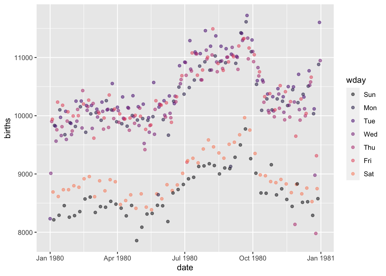
- The points split into two main groups based on the number of births each day. Explain in everyday terms what’s going on.
- There are some low-birth dates that are not weekends. Use wrangling to pull out those dates.
Answer:
Births |>
filter(births < 9400,
year == 1980,
wday %in% c("Mon", "Tue", "Wed", "Thu", "Fri"))Exercise 5.5
The n() adverbial wrangling shrinkage function counts the number of rows. It is unusual in that it doesn’t need any input; it is counting rows, not values in a variable.
- There is a simple relationship between the
rowscolumn in these two statements. What is that relationship?
- Replace
TinywithBigin your wrangling statements and explain if your answer to (1) still holds up.
Exercise 5.6 Each of these tasks can be performed using a single wrangling verb. For each task, write out the wangling step into which a data frame is piped.
Example: Find the average (mean) of a variable named brightness. Answer: summarize(mean(brightness))
Add a new column, to be named
rate, that is the ratio of two variables, X and Y, for each of the specimens. Answer:mutate(rate = X / Y)Sort the rows in descending order of a variable named
size. Answer:arrange(desc(size))Create a new data frame that includes only those rows that meet the criterion that the value of variable X be positive. Answer:
filter(X > 0)From a data frame with three categorical variables A, B, & C, and a quantitative variable X, produce an output that has the same specimens but only the variables A and X. Answer:
select(A, X)From a data frame with three categorical variables A,B, & C, and a quantitative variable X, produce an output named M that contains the maximum value of X over all the cases that have a given combination of A and B. Answer:
summarize(M - max(X), by = c(A, B)
Exercise 5.7 These questions refer to the ggplot2::diamonds data frame. Take a look at the codebook (using ?ggplot2::diamonds) so that you’ll understand the meaning of the tasks. (Motivated by Garrett Grolemund.)
Each of the following tasks can be accomplished by a statement of the form
For each task, give appropriate verbs and arguments to substitute in place of ..verb1.., ..args1.., ..args2.., and ..args3...
- Which color diamond is the largest on average (in terms of carats)?
Answer:
ggplot2::diamonds |>
summarize(mc = mean(carat), .by = color) |>
arrange(desc(mc)) |>
head(1)- Which clarity of diamond has the smallest average “table” per carat?
Answer:
ggplot2::diamonds |>
summarize(mt = mean(table), .by = clarity) |>
arrange(mt) |>
head(1)Exercise 5.8 The BNames data frame contains 1000 rows randomly selected from a US Social Security Administration data frame with almost 2 million rows that give, for each year since 1880, the names of babies born in that year and how many babies of each sex were given each name. (See babynames::babynames if you want the )
Here is BNames.
Each of a-e shows a random part of wrangling output when the input is BNames. Your task is to reconstruct the wrangling command to produce that output. (Hint: The total number of rows in the output can be an important clue.)
- Output table A (Only the
head()of the table is shown.)
| year | sex | name | n |
|---|---|---|---|
| 1894 | F | Fedora | 5 |
| 1952 | F | Donalda | 10 |
| 1990 | F | Josie | 363 |
| 1996 | F | Tiffani | 576 |
| 1980 | F | Teon | 5 |
| 2001 | F | Alexya | 35 |
Answer: Names |> arrange(sex) |> head()
- Output table B
| year | sex | name | n |
|---|---|---|---|
| 1894 | F | Fedora | 5 |
| 1952 | F | Donalda | 10 |
| 1990 | F | Josie | 363 |
| 1996 | F | Tiffani | 576 |
| 1980 | F | Teon | 5 |
| 2001 | F | Alexya | 35 |
Answer: Names |> filter(sex == "F") |> head()
- Output table C
| year | sex | name | n |
|---|---|---|---|
| 2001 | M | Lynwood | 8 |
| 2001 | M | Owais | 6 |
| 2001 | M | Mary | 13 |
| 2001 | M | Spence | 17 |
| 2001 | M | Seneca | 27 |
| 2002 | M | Jailon | 25 |
Answer: Names |> filter(sex == "M", year > 2000) |> arrange(year) |> head()
- Output table D (All of the table is shown.)
| sex | total |
|---|---|
| M | 52071 |
| F | 91940 |
Answer: Names |> summarize(total = sum(n), .by = sex)
- Output table E (All of the table is shown.)
| year | sex | total |
|---|---|---|
| 2016 | F | 763 |
| 2016 | M | 103 |
| 2017 | F | 59 |
| 2017 | M | 48 |
Answer:
Names |>
filter(year > 2015) |>
summarize(total = sum(n), .by = c(year, sex)) |>
arrange(year):::
Exercise 5.9 Imagine a data frame, Patients, with categorical variables name, diagnosis, sex, and quantitative variable age. Consider this data wrangling operation:
Patients |>
summarise(count=n(), meanAge = mean(age),
.by = c(**some variables**))Replacing some variables with each of the following, tell what variables will appear in the output
sexAnswer:count,meanAge,sexdiagnosisAnswer:count,meanAge,diagnosissex, diagnosisAnswer:count,meanAge,sex),diagnosisage, diagnosisAnswer:count,meanAge,age),diagnosisageAnswer:count,meanAge,age
Exercise 5.10 Here are three data frames, A, B, and C, with different organizations of the same data.
Format A
| Year | Algeria | Brazil | Columbia |
|---|---|---|---|
| 2000 | 7 | 12 | 16 |
| 2001 | 9 | 14 | 18 |
Format B
| Country | Y2000 | Y2001 |
|---|---|---|
| Algeria | 7 | 9 |
| Brazil | 12 | 14 |
| Columbia | 16 | 18 |
Format C
| country | year | value |
|---|---|---|
| Algeria | 2000 | 7 |
| Algeria | 2001 | 9 |
| Brazil | 2000 | 12 |
| Columbia | 2001 | 18 |
| Columbia | 2000 | 16 |
| Brazil | 2001 | 14 |
- What are the variables in each table?
- What is the meaning of a case for each table? Here are some possible choices.
- A country
- A country in a year
- A year
Answer:
- The variables are:
- Table A: Year, Algeria, Brazil, Columbia
- Table B: Country, Y2000, Y2001
- Table C: Country, Year, Value
- The cases are:
- Table A: a year
- Table B: a country
- Table C: a country in a year
- Which data-frame format do you think would make it easiest to find the change from 2000 to 2001 for each country? How would you do it?
Answer:
Format B is the easiest for calculating the change from 2000 to 2001. All you need is to subtract the two columns:
Format_B |> mutate(change = Y2001 - Y2000)Exercise 5.11
The city of Minneapolis, Minnesota was one of the first to try “ranked choice” voting. In an ordinary election, each voter selects one candidate. In contrast, in ranked-choice voting, the voter selects a first choice, a second choice, and a third choice.
The Minneapolis2013 data frame available for this exercise records the votes from the 2013 mayoral election. Here is a random sample of 500 rows out of 80,101 altogether:
Warning in instance$preRenderHook(instance): It seems your data is too big for
client-side DataTables. You may consider server-side processing:
https://rstudio.github.io/DT/server.htmlIn tallying up the ballots, the first-choice candidates are tallied. If one candidate has a majority, she wins. If not, then the candidate with the smallest number of first-choice votes is eliminated. Any ballots marked with that candidate have the eliminated candidate struck out, and remaining candidates on that ballot are moved up one choice. This process is repeated over and over until one candidate has a first-choice majority.
- How many ballots are there?
Answer:
Minneapolis2013 |> nrow()[1] 80101- Who were the top 5 candidates in the Second vote selections?
Answer:
Minneapolis2013 |>
summarize(count = n(), .by = Second) |>
arrange(desc(count)) |>
filter(Second != "undervote") |>
head(5)- How many ballots are marked “undervote” in
- First choice selections?
- Second choice selections?
- Third choice selections?
Answer:
Minneapolis2013 |>
summarize(first = sum(First == "undervote"),
second = sum(Second == "undervote"),
third = sum(Third == "undervote"))- What are the top 3 combinations of First and Second vote selections? (That is, of all the possible ways a voter might have marked his or her first and second choices, which received the highest number of votes?)
Answer:
Minneapolis2013 |>
summarize(count = n(), .by = c(First, Second)) |>
arrange(desc(count)) |>
head()- Which
Precincthad the highest number of ballots cast?
Answer:
Minneapolis2013 |>
summarize(count = n(), .by = Precinct) |>
arrange(desc(count)) |>
head()Enrichment topics
Enrichment topic 5.1: Pivoting
In an earlier example, we used mutate() to compute a new column called GDPpercap by dividing two existing columns, GDP and pop. With mutate(), it’s easy to do calculations that involve two or more columns within the same row.
Now consider a similar sounding task, computing GDPgrowth by dividing, for each country separately, the 2020 GDP with the 1950 GDP. This cannot be done with a simple mutate() step because the information needed for the calculation is spread over two different rows. A clue to the difficulty is that there are not separate columns named, say, GDP2020 and GDP1950 that could be combined with a mutate() operation.
“Pivoting” is a data wrangling operation that reshapes a data frame. Understanding pivoting is essential for the professional data scientist. But, like the construction of compound wrangling statements in general, mastery comes with experience. You won’t need to master pivot to study these Lessons, but we do use it behind the scenes in some of the demonstrations. Mainly, it’s worthwhile to learn a little about pivoting in order better to appreciate how data wrangling uses a small number of general-purpose operations to accomplish a huge variety of tasks.
Consider a data frame for which you want to turn information in different rows into a format with that information in different columns. That is, we’re going to take information from a single column in the original, and spread it between two (or more) columns in the output from the operation. Adding columns is effectively making a data frame “wider.” We can accomplish the GDPgrowth wrangling by pivoting from “longer” (that is, more rows) to “wider”. Like this:
This is a complicated command, so we will break it down argument by argument.
The first argument,
country, specifies the variable values that will label each row in the result. Even thoughcountryhas eight values, there are only four distinct values so the result will have four rows.The second argument,
values_from = c(GDP, pop), tells which columns we are going to make wider. Here, we are creating side-by-side columns for bothGDPandpop.The third argument,
names_from = year, tells what variable in the original will spread of the columns in the second argument. Sinceyearhas two distinct values (1950 and 2020), thevalues_fromcolumns will be split into two columns each. If year had three distinct values (say, 1980 as well as 1950 and 2020), then the splitting would be into three columns for each of thevalues_fromcolumns.
The pivoted data contains the same information as the original, but organized differently. The new organization makes it easy to do the GDPgrowth calculation, since now it is just the ratio of two columns:
As you might suspect, there is also a pivot_longer() operation, which merges columns rather than spreading them.