Galton |>
summarize(sd(height))8 Statistical thinking & variation
The central object of statistical thinking is variation. Whenever we consider more than one item of the same kind, , the items will likely differ from one another. Sometimes, the differences appear slight, as with the variation among fish in a school. Sometimes the differences are large, as with country-to-country variation in population size, land area, or economic production. Even carbon atoms—all made of identical protons, neutrons, and electrons—differ one from another in terms of energy state, bonds to molecular neighbors, and so on.
Expressed in terms of data frames, the “same kind” means the unit of observation, the type of specimen that occupies a row of a data frame.
In many settings, variation is inevitable. Example: The Earth is a spinning sphere. Consequently, the intensity of sunlight necessarily varies from place to place and time of day leading to wind and turbulence. Example: In biology, variation is a built-in feature of genetic mechanisms. results from genetic and environmental impacts, even at the level of a cell or even a virus. In human activities, sometimes variation is a nuisance as in industrial production; sometimes it provides important structure as with the days of the week and seasons of the year; sometimes—as in art—it is encouraged.
In the same era, the increased use of time-keeping in navigation and the need to make precise land surveys across large distances led to detailed astronomical observations. The measurements of the positions and alignment of stars and planets from different observatories were slightly inconsistent even when taken simultaneously. Such inconsistencies were deemed to be the result of error. Consequently, the “true” position and alignment was considered to be that offered by the most esteemed, prestigious, and authoritative observatory.
After 1800, attitudes began to change—slowly. Rather than referring to a single authoritative source, astronomers and surveyors used arithmetic to construct an artificial summary by averaging the varying individual observations. A Belgian astronomer, Adolphe Quételet, started to apply the astronomical techniques to social data. Among other things, in the 1830s Quételet introduced the notion of a crime rate. At the time, this was counter-intuitive because there is no central authority that regulates the commission of crimes.
Up through the early 1900s, the differences between individual observations and the summary were described as “errors” and “deviations.” But the summary is built from the observations; any “error” in the observations must pass through, to some extent, to the summary.
In natural science and engineering, it became important to be able to measure the likely amount of “error” in a summary, for instance, to determine whether the summary is consistent or inconsistent with a hypothesis. Similarly, if Quételet was to compare crime rates across state boundaries, he needed to know how precise his measurement was.
To illustrate, suppose Quételet was comparing crime rates in France and England. If the summaries were exact, a simple numerical comparison would suffice to establish the differences. However, since summaries are not infinitely precise, it is essential to consider their imprecision in making judgments of difference.
The challenge for the student of statistics is to overcome years of training suggesting wrongly that you can compare groups by comparing averages. The averages themselves are not sufficient. Statistical thinking is based on the idea that variation is an essential component of comparison. Comparing averages can be misleading without considering the specimen-to-specimen variation simultaneously.
As you learn to think statistically, it will help to have a concise definition. The following captures much of the essence of statistical thinking:
Statistic thinking is the accounting for variation in the context of what remains unaccounted for.
As we start, the previous sentence may be obscure. It will begin to make more and more sense as you work through these successive Lessons where, among other things, you will …
- Learn how to measure variation;
- Learn how to account for variation;
- Learn how to measure what remains unaccounted for.
Measuring variation
Yet another style for describing variation—one that will take primary place in these Lessons—uses only a single-number. Perhaps the simplest way to imagine how a single number can capture variation is to think about the numerical difference between the top and bottom of an interval description. We are throwing out some information in taking such a distance as the measure of variation. Taken together, the top and bottom of the interval describe two things: the location of the values and how different the values are from one another. These are both important, but it is the difference between values that gives a pure description of variation.
Early pioneers of statistics took some time to agree on a standard way of measuring variation. For instance, should it be the distance between the top and bottom of a 50% interval, or should an 80% interval be used, or something else? Ultimately, the selected standard is not about an interval but something more fundamental: the distances between pairs of individual values.
To illustrate, suppose the gestation variable had only two entries, say, 267 and 293 days. The difference between these is \(267-293 = -26\) days. Of course, we don’t intend to measure distance with a negative number. One solution is to use the absolute value of the difference. However, for subtle mathematical reasons relating to the Pythagorean theorem, we avoid negative numbers by using the square of the difference, that is, \((293 - 267)^2 = 676\) days-squared.
To extend this straightforward measure of variation to data with \(n > 2\) is simple: look at the square difference between every possible pair of values, then average. For instance, for \(n=3\) with values 267, 293, 284, look at the differences \((267-293)^2, (267-284)^2\) and \((293-284)^2\) and average them! This simple way of measuring variation is called the “modulus” and dates from at least 1885. Since then, statisticians have standardized on a closely related measure, the “variance,” which is the modulus divided by \(2\). Either one would have been fine, but honoring convention offers important advantages; like the rest of the world of statistics, we’ll use the variance to measure variation.
Variance as pairwise-differences
Figure fig-explain-modulus is a jitter plot of the gestation duration variable from the Gestation data frame. The graph has no explanatory variable because we are focusing on just one variable: gestation. The range in the values of gestation runs from just over 220 days to just under 360 days.
Each red line in Figure fig-explain-modulus connects two randomly selected values from the variable. Some lines are short; the values are pretty close (in vertical offset). Some of the lines are long; the values differ substantially.
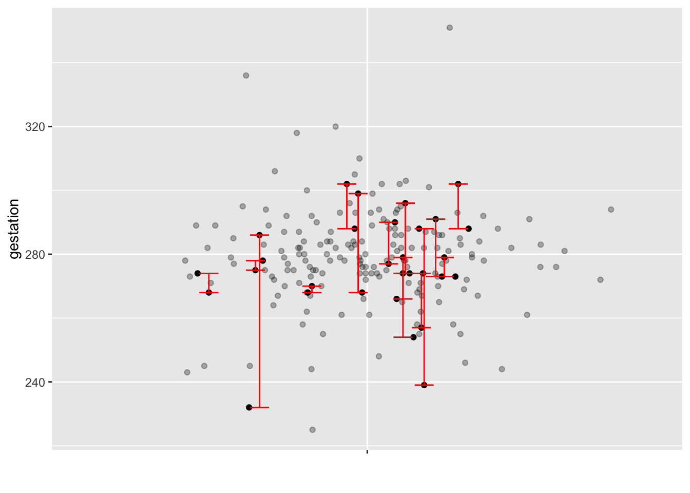
gestation duration (days) from the Gestation data frame. For every pair of dots, there is a vertical distance between them. To illustrate, a handful of pair have been randomly selected and their vertical difference annotated with a red line. The “modulus” is the average squared pairwise vertical difference, where the average is taken over all possible pairs (not just the ones annotated in red). The variance is the modulus divided by 2.
Only a few pairs of points have been connected with the red lines. To connect every possible pair of points would fill the graph with so many lines that it would be impossible to see that each line connects a pair of values.
The average square of the lines’ lengths (in the vertical direction) is called the “modulus.” We won’t use this word going forward in these Lessons; we accept that the conventional description of variation is the “variance.” Still, the modulus has a more natural explanation than the variance. Numerically, the variance is half the modulus.
Calculating the variance is straightforward using the var() function. Remember, var() is similar to the other reduction functions—e.g. mean() and median()—that distill multiple values into a single number. As always, the reduction functions need to be used within the arguments of a data wrangling function.of a set of data-frame rows to a single summary is accomplished with the summarize() wrangling command.
The variance is a numerical quantity whose units come from the variable itself. height in the Galton data frame is measured in inches. The variance averages the square of differences, so var(height) will have units of square-inches.
From variance to “standard deviation”
If you have studied statistics before, you have probably encountered the “standard deviation.” We avoid this terminology; it is long-winded and wrongly suggests a departure from the normal. Calculating the standard deviation involves two steps: first, find the variance; then take the square root. These two steps are automated in the sd() summary function.
A consequence of the use of squaring in defining the variance is the units of the result. gestation is measured in days, so var(gestation) is measured in days-squared.
Learning check 8.1
Use summary() to compute both the variance and standard deviation of the flipper length in the Penguins data frame.
After viewing the numbers, pipe the result into mutate() and do a simple calculation to demonstrate the numerical relationship between variance and standard deviation.
Exercises
Exercises
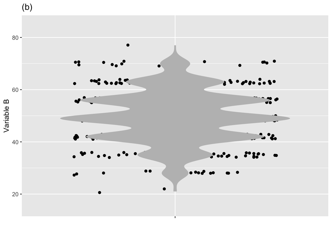
Exercise 8.1 The two jitter + violin graphs below show the distribution of two different variables, X and Y. Which variable has more variability?

Answer:
There is about the same level of variability in variable A and variable B. This surprises some people. Remember, the amount of variability has to do with the spread of values of the variable. In variable B, those values are have a 95% prediction interval of about 30 to 65, about the same as for variable A. There are two things about plot (b) that suggest to many people that there is more variability in variable B.
- The larger horizontal spread of the dots. Note that variable B is shown along the vertical axis. The horizontal spread imposed by jittering is completely arbitrary: the only values that count are on the y axis.
- The scalloped, irregular edges of the violin plot.
On the other hand, some people look at the clustering of the data points in graph (b) into several discrete values, creating empty spaces in between. To them, this clustering implies less variability. And, in a way, it does. But the statistical meaning of variability has to do with the overall spread of the points, not whether they are restricted to discrete values.
Exercise 8.2
- True or false: Variance refers to a data frame. Answer: False. Variance refers to a variable.
- Are “standard deviation” and “variance” the same thing? Answer: Almost. Standard deviation is the square root of variance. Many people prefer to use standard deviation because its units are the same as those of the variable. (Variance has the variable’s units squared. But variance has simpler mathematical properties.)
- True or false: Variance is about a single variable, not the relationship between two variables. Answer: True
Exercise 8.3 It is undeniably odd that the units of the variance are the square of the units of the variable for which the variance is calculated. For example, if the variable records height in units of meters, the variance of height will have units of square-meters. Sometime, the units of the variance have no physical meaning to most people. A case in point, if the variable records the temperature in degreesC, the variance will have units of degreesC2.
The odd units of the variance make it hard to estimate from a graph. But there is a trick that makes it straightforward.
Graph the values of the variable with a jittered point plot. The horizontal axis has no content because variance is about a single variable, not a pair of variables. The horizontal space is needed only to provide room for the jittered points to spread out.
Mark the graph with two horizontal lines. The space between the lines should include the central two-thirds of the points in the graph.
Find the intercept of each of the two lines with the vertical axis. We’ll call the two intercepts “top” and “bottom.”
Find the numerical difference between the top and the bottom. Divide this difference by 2 to get a “by-eye” estimate of the standard deviation. That is, the standard deviation is the length of a vertical line drawn from the mid-point of “top” and “bottom” to the top.
Square the standard deviation to get the value of the variance.
For each of the following graphics (in the style described in (1)), estimate the standard deviation and from that the variance of the data in the plot.
Warning in geom_jitter(point_ink = 0.3): Ignoring unknown parameters: `point_ink`
Ignoring unknown parameters: `point_ink`
Ignoring unknown parameters: `point_ink`
Ignoring unknown parameters: `point_ink`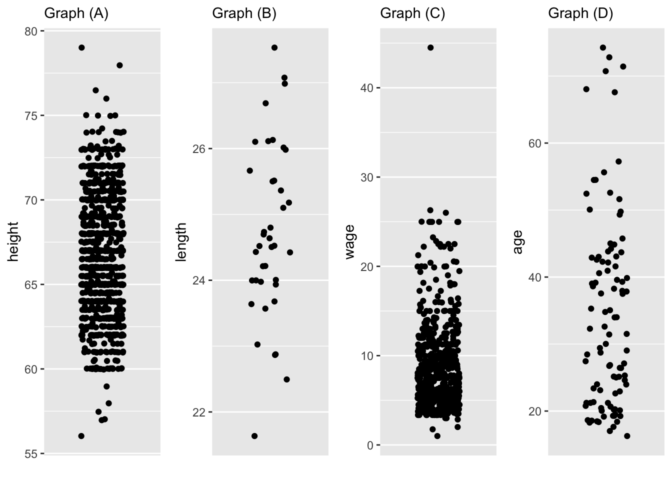
| Graph | Standard Dev. | Variance | units of sd | units of var |
|---|---|---|---|---|
| A | ||||
| B | ||||
| C | ||||
| D |
Exercise 8.4 Here is the variance of three variables from the Galton data frame.
Galton |>
summarize(vh = var(height), vm = var(mother), vf = var(father))| vh | vm | vf |
|---|---|---|
| 12.8373 | 5.322365 | 6.102164 |
All three variables—height, mother, father—give the height of a person. The height variable is special only because the people involved are the (adult-aged) children of the respective mother and father.
Height is measured in inches in
Galton. What are the units of the variances? Answer: Variance has the units of the square of the variable. In this case, that’s “square-inches.”Can you tell from the variances which group is the tallest: fathers, mothers, or adult children? Answer: Variance is about the differences between pairs of values in a variable. It does not have anything to say about whether the values are high or low, just about how they differ one to another.
Mothers and fathers have about the same variance. Yet the heights of the children have a variance that is more than twice as big. Let’s see why this is.
As you might expect, the mothers are all females and the fathers are all males. But the children, whose heights are recorded in heights, are a mixture of males and females. So the large variance, 12.8 square-inches, is a combination of the systematic variation between males and females and the person-to-person variation within each group.
Galton |>
  mutate(hdev = height - mean(height), .by = sex) |>
summarize(v_sex_adjusted = var(hdev), .by = sex)| sex | v_sex_adjusted |
|---|---|
| M | 6.925288 |
| F | 5.618415 |
Because the data have been grouped by sex, the mean(height) is found separately for males and females.
- The table just calculated gives the variance among the female (adult-aged) children and the variance among the male (adult-aged) children. Compare it to the variances for the fathers and mothers,
vmandvffrom the calculation made at the start of this exercise.
The variance calculations made using summarize(), var() and .by = sex can be done another way using regression modeling.
Galton |> model_train(height ~ sex) |>
  model_eval() |>
  summarize(var(.resid), .by = sex)
Using training data as input to model_eval().| sex | var(.resid) |
|---|---|
| M | 6.925288 |
| F | 5.618415 |
- Explain what the variance of the residual has to do with the variance of the sexes separately. Answer: It is roughly the average separate variances.
Exercise 8.5 Consider these calculations of the variation in age in the Whickham data frame:
Whickham |> summarize(var(age))| var(age) |
|---|
| 303.8756 |
Whickham |> summarize(var(age - 5))| var(age - 5) |
|---|
| 303.8756 |
Whickham |> summarize(var(age - mean(age)))| var(age - mean(age)) |
|---|
| 303.8756 |
Explain why the answers are all the same, even though different amounts are being subtracted from age?
Answer:
Variance is about the differences between pairs of values in a variable. Adding or subtracting the same quantity to all values does not change any of the differences between them.
Exercise 8.6
- Some by hand calculation of variance.
- Units of variance in various settings.
- Variance by eye
Enrichment topics
Enrichment topic 8.1: Instructor note: Measuring variation
Instructors and some students will bring their previous understanding of the measurement of variation to this section. They will likely be bemused by the presentation in this Lesson. First, this Lesson gives prime billing to the “variance” (rather than the “standard deviation”). Second, the calculation will be done in an unconventional way.
There are three solid reasons for the departure from the convention. I recognize that the usual formula is the correct, computationally efficient algorithm for measuring variation. That algorithm is usually presented algebraically, even though many students do not parse algebraic notation of such complexity:
\[{\large s} \equiv \sqrt{\frac{1}{n-1} \sum_i \left(x_i - \bar{x}\right)^2}\ .\] The first step in the conventional calculation of the standard deviation \(s\) is to find the mean value of \(x\), that is
\[{\large\bar{x}} = \frac{1}{n} \sum_i x_i\] For those students who can parse the formulas, the clear implication is that the standard deviation depends on the mean.
The mean and the variance (or its square root, the standard deviation) are independent. Each can take on any value at all without changing the other. The mean and the variance measure two utterly distinct characteristics. The method shown in the text avoids making the misleading link between the mean and the variance.
As well, the text’s formulation avoids any need to introduce the distracting \(n-1\). The effect of the \(n-1\) is already accounted for in the text’s simple averaging.
Finally, working directly with the variance verbally reminds us that it is a measure of variation, avoids the obscure and oddball name “standard deviation,” and simplifies the accounting of variation by removing the need to square standard deviations before working with them.
Instructors should point out to students that the units of the variance are not those of the mean. For instance, the variance of a set of heights will have units height2: area. It’s reasonable for the units to differ, just as units for gas volume and pressure vary. Variances and means are different quantities measured in different ways.