Galton |>
  model_train(height ~ mother + father + sex) |>
  coef()
(Intercept) mother father sexM
15.3447600 0.3214951 0.4059780 5.2259513 A food market will give you a sample of an item on sale: a tiny cup of a drink or a taste of a piece of fruit or other food item. Laundry-detergent companies sometimes send out a sample of their product in the form of a small foil packet suitable for only a single wash cycle. Paint stores keep small samples on hand to help customers choose from among the possibilities. A fabric sample is a little swatch of cloth cut from a a bigger bolt that a customer is considering buying. A dictionary definition of sample is, “a small part or quantity intended to show what the whole is like.”
In contrast, in statistics, a sample is always a collection of multiple items. The individual items are specimens, each one recorded in its own row of a data frame. The entries in that row record the measured attributes of that specimen.
The collection of specimens is the sample. In museums, the curators put related specimens—fossils or stone tools—into a drawer or shelf. Statisticians use data frames to hold their samples. A “sample” is akin to words like “a herd,” “a flock,” “a pack,” or “a school,” each of which refers to a collective. A single fish is not a school; a single wolf is not a pack. Similarly, a single row is not a sample but a specimen.
The dictionary definition of “sample” uses the word “whole” to describe where the sample comes from. Similarly, a statistical sample is a collection of specimens selected from a larger “whole.” Traditionally, statisticians have used the word “population” as the name for the “whole.” “Population” is a good metaphor; it’s easy to imagine the population of a state being the source of a sample in which each individual is a specific person. But the “whole” from which a sample is collected does not need to be a finite, definite set of individuals like the citizens of a state. For example, you have already seen how to collect a sample of any size you want from a DAG.
An example of a sample is the data frame Galton, which records the heights of a few hundred people sampled from the population of London in the 1880s.
Our modus operandi in these Lessons takes a sample, stores the sample one specimen per row a data frame and summarizes the whole sample in the form of one or more numbers: a “sample summary.” Typically, the sample summary is the coefficients of a regression model, but it might be something else such as the mean or variance of a variable.
As a concrete example, consider this sample summary of Galton.
The summary includes two numbers, the variance and the mean of the height variable. Each of these numbers is called a “sample statistic.” In other words, the summary consists of two sample statistics.
There can be many ways to summarize a sample. Here is another summary of Galton:
Galton |>
model_train(height ~ mother + father + sex) |>
coef()(Intercept) mother father sexM
15.3447600 0.3214951 0.4059780 5.2259513 This summary has four numbers, each of which is a regression coefficient. Here too, each of the regression coefficients is a “sample statistic.”
To understand samples and sampling, it helps to start with a collection that is not a sample. A non-sample data frame contains a row for every member of the literal, finite “population.” Such a complete enumeration—the inventory records of a merchant, the records kept of student grades by the school registrar—has a technical name: a “census .” Famously, many countries conduct a census of the population in which they try to record every resident of the country. For example, the US, UK, and China carry out a census every ten years.
In a typical setting, recording every possible observation unit is unfeasible. Such incomplete records constitute a “sample.” One of the great successes of statistics is the means to draw useful information from a sample, at least when the sample is collected with a correct methodology.
Sampling is called for when we want to find out about a large group but lack time, energy, money, or the other resources needed to contact every group member. For instance, unlike the 10-year census, France collects samples from its population at short intervals to collect up-to-date data while staying within a budget. The name used for the process—the recensement en continu (“rolling census”)—signals the intent. Over several years, the recensement en continu contacts about 70% of the population. As such, it is not a “census” in the narrow statistical sense.
Another example of the need to sample comes from quality control in manufacturing. The quality-control measurement process is often destructive: the measurement process consumes the item. In a destructive measurement situation, it would be pointless to measure every single item. Instead, a sample will have to do.
Collecting a reliable sample is usually considerable work. An ideal is the “simple random sample” (SRS), where all of the items are available, but only some are selected—completely at random—for recording as data. Undertaking an SRS requires assembling a “sampling frame,” essentially a census. Then, with the sampling frame in hand, a computer or throws of the dice can accomplish the random selection for the sample.
Understandably, if a census is unfeasible, constructing a perfect sampling frame is hardly less so. In practice, the sample is assembled by randomly dialing phone numbers or taking every 10th visitor to a clinic or similar means. Unlike genuinely random samples, the samples created by these practical methods do not necessarily represent the larger group accurately. For instance, many people will not answer a phone call from a stranger; such people are underrepresented in the sample. Similarly, the people who can get to the clinic may be healthier than those who cannot. Such unrepresentativeness is called “sampling bias.”
Professional work, such as collecting unemployment data, often requires government-level resources. Assembling representative samples uses specialized statistical techniques such as stratification and weighting of the results. We will not cover the specialized methods in this introductory course, even though they are essential in creating representative samples. The table of contents of a classic text, William Cochran’s Sampling techniques shows what is involved.
All statistical thinkers, whether experts in sampling techniques or not, should be aware of factors that can bias a sample away from being representative. In political polls, many (most?) people will not respond to the questions. If this non-response stems from, for example, an expectation that the response will be unpopular, then the poll sample will not adequately reflect unpopular opinions. This kind of non-response bias can be significant, even overwhelming, in surveys.
Survival bias plays a role in many settings. The mosaicData::TenMileRace data frame provides an example, recording the running times of 8636 participants in a 10-mile road race and including information about each runner’s age. Can such data carry information about changes in running performance as people age? The data frame includes runners aged 10 to 87. Nevertheless, a model of running time as a function of age from this data frame is seriously biased. The reason? As people age, casual runners tend to drop out of such races. So the older runners are skewed toward higher performance.
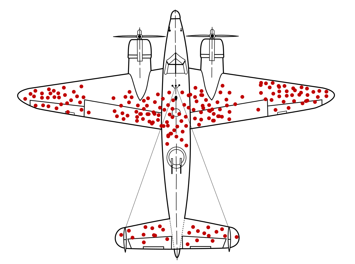
An inspiring story about dealing with survival bias comes from a World War II study of the damage sustained by bombers due to enemy guns. The sample, by necessity, included only those bombers that survived the mission and returned to base. The holes in those surviving bombers tell a story of survival bias. Shell holes on the surviving planes were clustered in certain areas, as depicted in Figure 19.1. The clustering stems from survivor bias. The unfortunate planes hit in the middle of the wings, cockpit, engines, and the back of the fuselage did not return to base. Shell hits in those areas never made it into the record.
For the last 20 years, conventional wisdom has held that lower socio-economic status families talk to their children less than higher status families. The quoted number is a gap of 30 million words per year between the low-status and high-status families.
The 30-million word gap is due to … mainly, sampling bias. This story from National Public Radio explains some of the sources of bias in counting words spoken. More comes from the original data being collected by spending an hour with families in the early evening. That’s the time, later research has found, that families converse the most. More systematic sampling, using what are effectively “word pedometers,” puts the gap at 4 million words per year.
Usually we work with a single sample, the data frame at hand. As always, the data consists of signal combined with noise. To see the consequences of sampling on summary statistics such as model coefficients, consider a “thought experiment.” Imagine having multiple samples, each collected independently and at random from the same source and stored in its own data frame. Continuing the thought experiment, calculate sample statistics in the same way for each data frame, say, a particular regression coefficient. In the end, we will have a collection of equivalent sample statistics. We say “equivalent” because each individual sample statistic was computed in the same way. But the sample statistics, although equivalent, will differ one from another to some extent because they come from different samples. Sample by sample, the sample statistics vary one to the other. We call such variation among the summaries “sampling variation .”
The proposed thought experiment can be carried out. We just need a way to collect many samples from the same data source. To that end, we use a data simulation as the source. The simulation provides an inexhaustible supply of potential samples. Then, we will calculate a sample statistic for each sample. This will enable us to see sampling variation directly.
Our standard way of measuring the amount of variation is with the variance. Here, we will measure the variance of a sample statistic from a large set of samples. To remind us that the variance we calculate is to measure sampling variation, we will give it a distinct name: the “sampling variance.”
Pay careful attention to the “ing” ending in “sampling variation” and “sampling variance. The phrase”sample statistic” does not have an “ing” ending. When we use the “ing” in “sampling,” it is to emphasize that we are looking not just at a single sample, but at the variation in the sample statistic from one sample to another.
The simulation technique will enable us to witness essential properties of the sampling variance, particularly how it depends on sample size \(n\).
We will use sim_02 as the data source, but the same results would be found with any other simulation.
print(sim_02)Simulation object
------------
[1] x <- rnorm(n)
[2] a <- rnorm(n)
[3] y <- 3 * x - 1.5 * a + 5 + rnorm(n)You can see from the mechanisms of sim_02 that the model y ~ x + a will, ideally, produce an intercept of 5, an x-coefficient of 3, and an a-coefficient of -1.5. By “ideally,” we mean that a model trained on the simulated data will give the those coefficients if the sample size is large enough.
Run Listing 19.1 many times and observe the model coefficients. Each time you run the simulation, you are getting a new random sample from the simulation. Since the sample differs from run to run, the fitted model coefficients also vary from run to run. This is sampling variation.
To see sampling variation directly, we need to compare multiple samples. If you followed the instructions of the previous paragraph—it isn’t too late!—you saw the coeficients vary. In the next chunk, you are going to automate the process of making new samples and collecting the coefficients, so that you can easily display the variation.
In Figure 19.2, the sampling variation is evident in the spread of coefficient values for each term.
A hallmark of sampling variation is that it gets smaller as the sample size gets larger. Repeat the trials in Figure 19.2 but with a sample of size n = 250 rather than n = 25.
According to sim_02, the coefficients used in forming y from x and a are:
Figure 19.2 shows that the individual trials deviate somewhat from these values, but the distribution as a whole is centered on the values from the simulation formula.
Use wrangling to calculate the variance across trials for each term.
This way of quantifying the amount of sampling variation is called the “sampling variance.” (Note the ing on sampling.)
The hallmark of sampling variability is that it gets smaller as the sample size get’s larger. Write down the three variances of the coefficients from the sample size n = 25. Then go back to Figure 19.2 and repeat the trials and the calculation of sampling variance for sample size n = 250. How much smaller is the sampling variance in n = 250 compared to n = 25?
Now try the same thing, but with n = 2500. The is a general pattern of relationship between the sampling variation and the sample size. Describe it quantitatively like this: “When the sample size is increased by a factor of 10, the sampling variation decreases by a factor of ……..”
Often, statisticians prefer to report the square root of the sampling variance. This has a technical name in statistics: the standard error. The “standard error” is an ordinary standard deviation in a particular context: the standard deviation across random trials. The words standard error should be followed by a description of the summary and the size of the individual samples involved. Here, the correct statement is, “The standard error of the Intercept coefficient from a sample of size \(n=25\) is around 0.2.”
It is easy to confuse “standard error” with “standard deviation.” Adding to the potential confusion is another related term, the “margin of error.” We can avoid this confusion by using an interval description of the sampling variation. You have already seen this: the confidence interval (as computed by conf_interval()). The confidence interval is designed to cover the central 95% of the sampling distribution. (See Lesson -Chapter 20.)
Take-home point: The larger the sample size, the smaller the sampling variance of a model coefficient or other summary statistic. For a sample of size \(n\), the sampling variance will be proportional to \(1/n\). Or, in terms of the standard error: For a sample size of \(n\), the standard error will be proportional to \(1/\sqrt{\strut n}\).
In Lesson 20 we will see how to use the dependence of sample variation on \(n\) into a way to estimate the amount of sampling variation from a single sample. This is what will enable us to more from simulated data to actual data.
Exercise 19.1
Pick up on the independent noise_sim from the simulation chapter. Have them explore the R2 and x-coefficient with different sample sizes.
noise_sim <- datasim_make(
  x <- rnorm(n),
  y <- rnorm(n)
)
Mod <- noise_sim |>take_sample(n=1000000) |>
model_train(y ~ x)
Mod |> conf_interval()| term | .lwr | .coef | .upr |
|---|---|---|---|
| (Intercept) | -0.001221 | 0.0007392 | 0.002699 |
| x | -0.001943 | 0.0000145 | 0.001973 |
Mod |> R2()| n | k | Rsquared | F | adjR2 | p | df.num | df.denom |
|---|---|---|---|---|---|---|---|
| 1e+06 | 1 | 0 | 0.0002112 | -1e-06 | 0.9884 | 1 | 1e+06 |
Exercise 19.2
TURN THIS EXAMPLE, from the point-plot chapter, into an EXAMPLE of how more data reveals more detail. Or maybe it should go in the confidence interval chapter.
In the panels below, we select random samples of the 10,000 biggest cities. The panel labeled n=100 has just one hundred cities, while n=500 has five hundred, and so on.
One principle of statistics: when displaying a pattern in data, a larger sample size lets you see more detail. Here, the pattern is one you learned in geography class in elementary school; the detail is in the shape of coastlines. For the most part, the patterns we consider in these Lessons are more abstract: relationships between variables.


Exercise 19.3
MAKE A PROJECT OF THE RUNNING DATA
Cross-sectional versus longitudinal. We can see the survival bias in the runners data by taking a different approach to the sample: collecting data over multiple years and tracking individual runners as they age.