1 Data frames
The origin of recorded history is, literally, data. Five-thousand years ago, in Mesopotamia, the climate was changing. Retreating sources of irrigation water called for an organized and coordinated response, beyond the scope of isolated clans of farmers. To provide this response, a new social structure – government – was established and grew. Taxes were owed and paid, each transaction recorded. Food grain had to be measured and stored, livestock counted, trades and shipments memorialized.
Writing emerged as the technological innovation to keep track of all this. We know this today because memoranda were incised by stylus on soft clay tablets and baked into permanence. When the records were no longer needed, they were recycled as building materials for the growing settlements and cities. Archaeologists started uncovering these tablets more than 100 years ago, spending decades to decipher the meaning of the stylus marks in clay.
The writing and record-keeping technology developed over time: knots in string, wax tablets, papyrus, vellum, paper, and computer memory. Making sense of the records has always required literacy, deciphering marks according to the system and language used to represent the writer’s intent. Today, in many societies, the vast majority of people have been taught to read and write their native language according to the accepted conventions.
Conventions of record keeping diverge from those of everyday language. For instance, financial transaction records must be guarded against error and fraud. Starting in the thirteenth century, financial accountants adopted a practice—double-entry bookkeeping—that has no counterpart in everyday language.
“Double-entry bookkeeping,” records each transaction twice, in two different places, in the form of a credit to an account and a debit from another account.
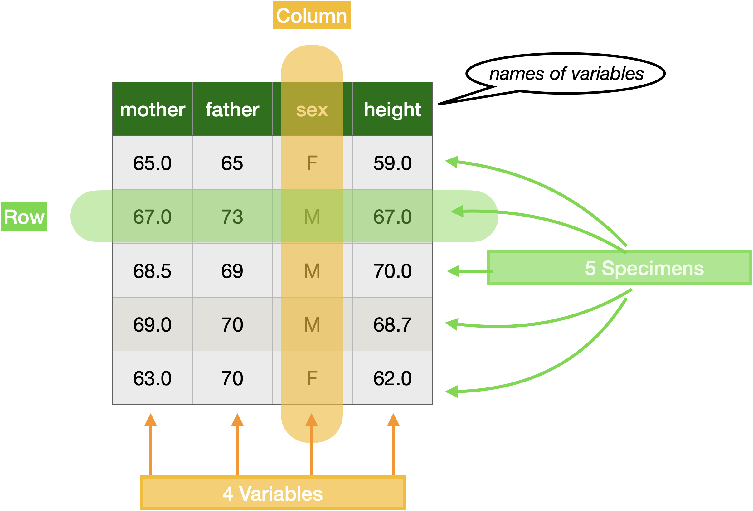
Modern conventions make working with data more accessible and more reliable. Of primary interest to us in these Lessons is the organization provided by a data frame , a structure for holding data as exemplified in Figure fig-data-frame-schematic.
Words marked with , as in data frame , have a definition in the Glossary. Click on the to pop up the definition.
Comment on the data in Figure fig-data-frame-schematic
The display in Figure fig-data-frame-schematic shows a small part of a larger data frame holding observations collected by statistician Francis Galton in the 1880s. I will use this data frame repeatedly across these lessons because of the outsized historical role the data played in the development of statistical methodology. The context for the data collection was Galton’s attempt to quantify the heritability of biological traits. The particular trait of interest to Galton (probably because it is easily measured) is human stature. Galton recorded the heights of full-grown children and their parents.
The word “variable” is appropriate. The values in a variable vary from one from one row to another. Other English words with the same root include “variation,” “variety,” and even “diversity.”
The row-and-column organization of a data frame is reminiscent of a spreadsheet. However, data frames have additional organizational requirements that typical spreadsheet software does not enforce. The term “tidy data” emphasizes that these requirements are being met.
Each variable must consist of the same kind of individual entries. For example, the
mothervariable consists of numbers: a quantity. In this case, the quantity is the mother’s height in inches. It would not be legitimate for an entry inmotherto be a word or to be a height in meters or something else entirely, for instance, a blood pressure.Each row represents an individual real-world entity. For the data frame shown in Figure fig-data-frame-schematic, each row corresponds to an individual, fully-grown child. We use the term “unit of observation” to refer to the kind of entity represented in each row. All rows in a data frame must be the same kind of unit of observation. It would not be legitimate for some rows to individual people while others refer to something different such as a house or family or country. If you wanted to record data on families, you would need to create a new data frame where the unit of observation is a family.
We use the word “specimen” to refer to an individual instance of the unit of observation. A data frame is a collection of specimens. Each row represents a unique specimen.
The unit of observation in Figure fig-data-frame-schematic is a full-grown child. The fifth row in that data frame refers to a unique young woman in London in the 1880s (whose name is lost to history). By using the word “specimen” to refer to this woman, we do not mean to dehumanize her. However, we need a phrase that can be applied to a single row of any data frame, whatever its unit of observation might be: a shipping container, a blood sample, a day of ticket sales, and so on.
The collection of specimens comprised by a data frame is often a “sample” from a larger group of the units of observation. Galton did not measure the height of every fully-grown child in London, England, the UK, or the World. He collected a sample from London families. Sometimes, a data frame includes every possible instance of the unit of observation. For example, a library catalog lists comprehensively the books in a library. Such a comprehensive collection is called a “census .”
Example: New-born babies
The US Centers for Disease Control (CDC) publishes a “public use file” each year, a data frame where the unit of observation is an infant born in the US. The many variables include the baby’s weight and sex, the mother’s age, and the number of prenatal care visits during the pregnancy. The published file for 2022 contains 3,699,040 rows; that is the number of (known) births in 2022. As such, the CDC data constitutes a census rather than a sample.
For demonstration purposes, these Lessons make available a random sample of size 20,000 of the CDC public-use file. The data frame containing the sample is named Births2022.
Computing with R
The computer is the essential tool for working with data. Traditionally, mathematics education has emphasized carrying out procedures with paper and pencil, or perhaps a calculator. Many statistics textbooks have inherited this tradition. This has a very unhappy consequence: the methods and concepts in those books are mainly limited to those developed before computers became available. This rules out using or understanding many of the concepts and techniques that form the basis for modern applied statistics. For example, news reports about medical research often include phrases like “after adjusting for …” or use techniques such as “logistic regression” or other machine-learning approaches. Traditional beginning statistics text are silent about such things.
There are many software packages for data and statistical computing. These Lessons use one of the most popular and powerful statistics software systems: R, a free, open-source system that is used by millions of people in many diverse disciplines and workplaces. It is also highly regarded in business, industry, science, and government. Fortunately, you do not have to learn the R language; you need only a couple dozen R expressions to work through all these Lessons.
To help to make getting started with R as simple as possible, Lessons provides interactive R computing directly in the text. This takes the form of R “chunks” that display one or more R commands in an editable box. When you press “Run Code” in a chunk, the command is evaluated by R and the results of the command displayed.
We will mostly be working with data frames that have already been uploaded to R and can be accessed by name. For instance, we mentioned above the Births2022 data frame.
Here’s a basic R command that displays the first rows of a data frame. Such a display can be useful to orient yourself to how the data frame is arranged. Let’s do this for Births2022:
Since there are 38 variables and 20,000 rows in Births2022, the output from Births2022 |> head() is truncated to fit reasonably on the page.
Other commands in these Lessons will have the same general layout as the one above. For instance,
- How many rows in a data frame?
- What are the names of the variables?
These commands each consist of three elements:
- The name of a data frame at the start of the command.
- The name of an action to perform followed immediately by parentheses.
- In between (1) and (2) is some punctuation:
|>. The shape of the punctuation reflects its purpose: the data frame on the left is being sent as an input to the task named on the right.
Tip
Create R commands in the following chunk to answer these questions.
- How many rows are in the
Galtondata frame? - What are the names of the variables in the
Galtondata frame? - What is the value of the variable
motherin the third row ofGalton?
T get started … Replace the ..data_frame with the name of the data frame, and ..action.. with the name of the action you want to perform.
- The relevant actions to choose from are
nrow,names, andhead. - Remember to leave the parentheses after the action name.
- Remember to leave the pipe symbol—
|>— between the data frame name and the action name.
Tip 1.1
The following R command is intended to display the names of the variables in the Galton data frame. But something is broken! So if you run the code—Try it!—you will get an error message.
Fix the command to carry out the intended calculation.
- Check spelling! There are two spelling mistakes in the original version of the command.
- Something about parentheses is very much like the story of Noah’s Ark.
Types of variables
Every variable in a tidy data frame has a type. The two most common types—and really, the only two types we need to work with— are quantitative and categorical.
Quantitative variables record an “amount” of something. These might just as well be called “numerical” variables.
Categorical variables typically consist of letters. For instance, the
sexvariable in Figure fig-data-frame-schematic contains entries that are either F or M. In most of the data we work with in these Lessons, there is a fixed set of entry values called the levels of the categorical variable. The levels ofsexare F and M.
To illustrate, the following command selects five of the 38 variables for display. Even though you won’t encounter such data wrangling until Lesson sec-wrangling, you may be able to make sense of the command. (If not, don’t worry!)
Births2022 data.
You can see that mage, duration, and weight are numerical. In contrast, meduc and anesthesia are categorical.
The values of each categorical variable come from a set of possibilities called levels. To judge from the display in Active R chunk lst-births-5, the possible levels for the anesthesia variable are Y and N. The meduc variable has different levels: Assoc, HS, Masters show up in the five rows from Active R chunk lst-births-5. The NA in the second row of meduc stands for “not available” and indicates that no value was recorded. You will encounter such NAs frequently in working with data.
Looking at a few rows of a data frame with head() is a simple way to get oriented, but there is no reason why every level of a categorical variable will appear. The count() function provides an exhaustive listing of every level of a categorical variable, like this:
count() function lists all of the levels of the variable named. It also counts how many times each level appears.
Tip 1.1
Active R chunk lst-births-count shows what is the point of the parentheses that follow a function name. The information given inside the parentheses is used to specify the details of the action the function will undertake. Such details are called the arguments of the function. For count(), the argument specifies the name of the variable for which counting will be done.
It’s natural to use the words “give” and “take” when it comes to arguments. You give a value for the argument. In Active R chunk lst-births-count, the given argument is meduc. The function takes an argument, meaning that it provides you an opportunity to give a value for that argument.
Some functions can take more than one argument. For example, the select() function in Active R chunk lst-births-5 can take any number of arguments, each of which is the name of a variable in the data frame provided by the pipe. When there are multiple arguments, successive arguments are separated by a comma.
Tip 1.2
Although count() is usually applied to a categorical variable, it is technically possible to count() the different values of a quantitative variable. Sometimes this is informative, sometimes not.
A. Apply count() to the baby’s weight variable. Why are their so many levels, and so few specimens per level?
B. Apply count() to the baby’s apgar5 variable. How many different levels are there? Look up “APGAR score,” named after the pioneering physician Dr. Virginia Apgar, to understand why.
Tip 1.3
The codebook
How are you to know for any given data frame what constitutes the unit of observation or what each variable is about? For instance, in Births2022 there are variables duration and weight. The duration of what? The weight of what? This information, sometimes called metadata , is stored outside the data frame. Often, the metadata is contained in a separate documentation file called a codebook .
To start, the codebook should make clear what is the unit of observation for the data frame. For instance, we described the unit of observation for the data frame shown in Figure fig-data-frame-schematic as a fully grown child. This detail is important. For instance, each such child—each specimen—can appear only once in the data frame. In contrast, the same mother and father might appear for multiple specimens, namely, the siblings of the child.
In the Births2020 data frame, the unit of observation is a newborn baby. If a birth resulted in twins, each of the two babies will have its own row. In contrast, imagine a data frame for the birth mothers or another for prenatal care visits. Each mother could appear only once in the birth-mothers frame, but the same mother can appear multiple times in the prenatal care data frame.
For quantitative variables, the relevant metadata includes what the number refers to (e.g., mother’s height mheight or baby’s weight, weight) and the physical units of that quantity (e.g., inches for mheight or grams for weight).
For categorical variables, the metadata should describe the meaning of each level in as much detail as necessary.
Example (cont.): CDC births codebook
The codebook for the original CDC data is a PDF document entitled “User Guide to the 2022 Natality Public Use File.” You can access it on the CDC website. The sample Births2022 has more compact documentation. You can see the documentation of most any R data frame by using ? followed by the name of the data frame.
Tip 1.4
What is the most common attendant at the births recorded in Births2022?
- Look back at Active R chunk lst-births-count.
Exercises
Activity 1.1 Historians have access to the physical notebook in which Francis Galton originally recorded the data on heights shown in Table tbl-galton-dataframe. Galton’s data is given as tables: intended for human eyes. (Galton worked well before the invention of modern computing.)
Here is part of Galton’s notebook holding the height data table:
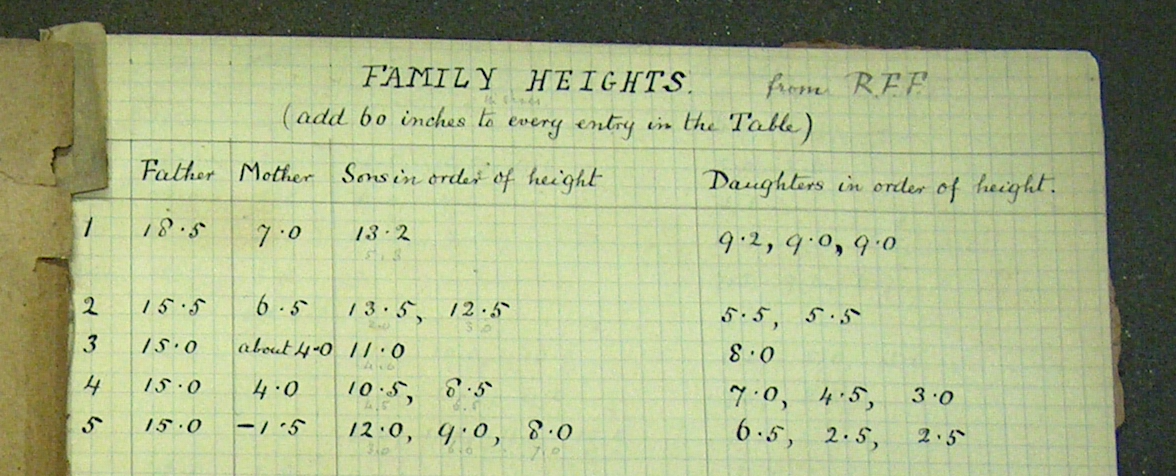
Describe the ways in which Galton’s data organization differs from that of a data frame.
Activity 1.2
In this exercise, you’ll examine two different data frames that are about births of babies. These are Births78 and Natality_2014. You can get the codebook for either in the usual way: ?Births78 or ?Natality_2014.
Births78andNatality_2014have utterly different units of observation. What are the units of observation of each of these two data frames? (Hint: Look at the documentation for each of them in the usual way.)What are the levels of the categorical variable
wdayinBirths78? (Hint: Usehead()orcount().)One deficiency in the documentation of
Natality_2014is that the documentation for variabledwgt_rdoes not say what units (if any) the values are in. The values are numbers in the range 100 to 400. To judge from the documentation, what are the units ofdwgt_r? (Hint: Other than to look at the documentation, you don’t need R to answer this one, just common sense.)
Activity 1.3
The documentation for the Galton data frame is not well written. It refers to 898 “observations”, but this is not really the unit of observation.
Look at the Galton data frame to determine which of these is the unit of observation:
- a family
- an individual person
- a father
- a mother
- the parents as a couple
Give the specific reasons why the other choices are incorrect.
Answer: There is data about the family, but in some cases a family appears in more than one row, so it cannot be the unit of observation. The same holds true for iii, iv, and v.
Activity 1.4 The unit of observation in the mosaicData::KidsFeet data frame is a 3rd- or 4th-grade student in the elementary school attended by a statistician’s daughter. You can see the first few rows by giving the R command
- For each variable, say whether “categorical” or “quantitative” gives the better description of the variable’s type.
Answer: birthmonth, birthyear, length, and width are quantitative. The others are categorical.
- The
birthmonthandbirthyearvariables are written with numerals, but this is due to deficiencies in the software used to record the data in the 1990s. Describe one way in whichbirthmonthdoes not behave arithmetically like a number. (Hint: Is 12/1987 close or far from 01/1988?)
Answer: Arithmetically, month 1 and month 12 are separated by 11 months. But in birthmonth this isn’t true, a 1 and a 12 can be adjacent.
Activity 1.5
Here are the first few rows of the Galton data frame. The unit of observation is a (fully grown) child.
Imagine the Francis Galton, who collected these data, was still alive and …
… wanted to add additional children to the data frame. Would this involve adding rows or adding columns? Answer: Additional specimens correspond to additional rows.
… wanted to add additional information about each child, for instance their favorite color or whether they ever had a broken bone. Would this involve adding rows or adding columns? Answer: Each additional type of information needs to be stored in its own column. So add variables
fav_colorandbroke_boneGive some examples of the likely levels for a variable like
fav_color. Answer: Green, Yellow, Red, Blue, …
Activity 1.6 The table below is from a so-called “population schedule” from the 1940 US Census. Column 1 indicates that the people listed live on N. Nevada Street. Columns 8 and 9 list the names of the individual people and their role in the household.
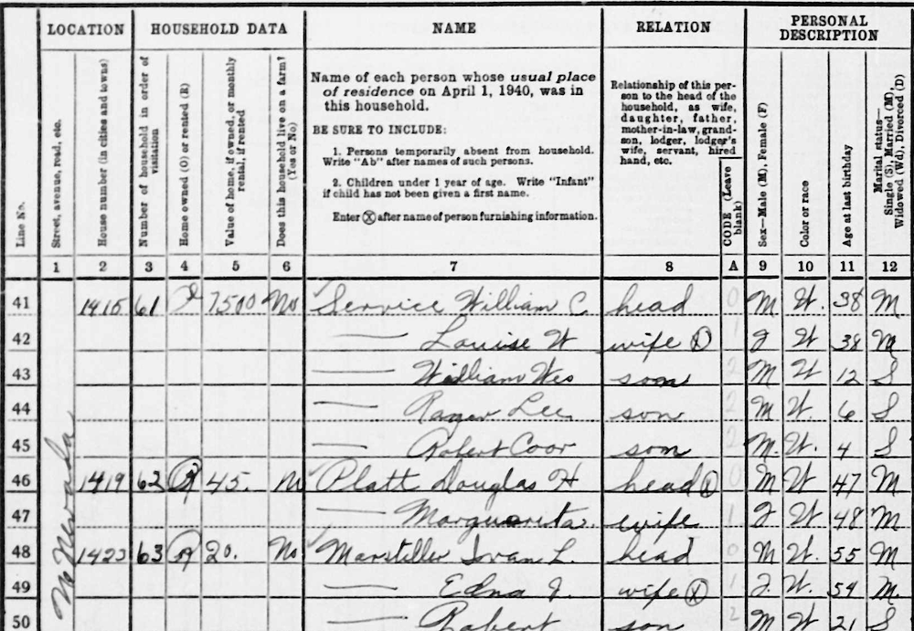
In 1940, principles of data organization were primitive. Using modern principles, raw data such as this would be arranged so that the order of the rows does not matter.
Explain why, in the 1940 table, the order of rows makes a big difference. For example, consider what would be changed about the data if, say, row 42 were moved to be between rows 47 and 48.
Answer: If row 42 were moved down by six rows, Louisa W. Service would become Louisa W. Platt, Douglas H Platt would become a bigamist with two wives, and William C Service would become a single parent! That’s inconsistent with the actual facts.
Activity 1.7
Many organizations, such as government agencies, provide access to data collected during their normal operations. For instance, New York City has an “open data” site that, among many other data frames, shows parking violations in the city over the last several years.
Using your web browser, go to the front page for the parking violation data: https://data.cityofnewyork.us/City-Government/Open-Parking-and-Camera-Violations/nc67-uf89. The front page provides several resources about the data, as well as a small preview of a handful of rows of the data frame. (Don’t try to read the data into R; it’s too big to be easily handled on a laptop computer.) Looking at the front page, answer these questions:
How many rows are in the data frame? Answer: This depends on the date you look at the data, but as of December 2023, there were over 107 million rows!
The third column is labelled “License Type.” Only two types—
PASandCOM—are shown in the first page of the data preview. Scroll down through the data preview until you have found three other license types. Which ones did you find? Answer: OMS, OMR, OMT appear within the first few pages.According to the front page, the unit of observation is an “Open Parking and Camera Violations [sic] Issued.” (Actually, the unit is a single violation.) The front page doesn’t use the term “unit of observation.” What term does it use instead? Answer: “Each row is a …”
Activity 1.8 Say what’s not tidy about this table.
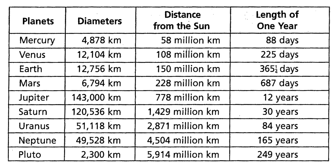
Answer:
- Units ought to be in the codebook not the data frame.
- The “length of year” variable is in a mixture of units. Some rows are (Earth) days, others are (Earth) years.
- The numbers have commas, which are intended for human consumption. Data tables are for machine consumption and the commas are a nuisance.
- The \(\frac{1}{4}\) in the “length of year” column is not a standard computer numeral. Write 365.25 instead.
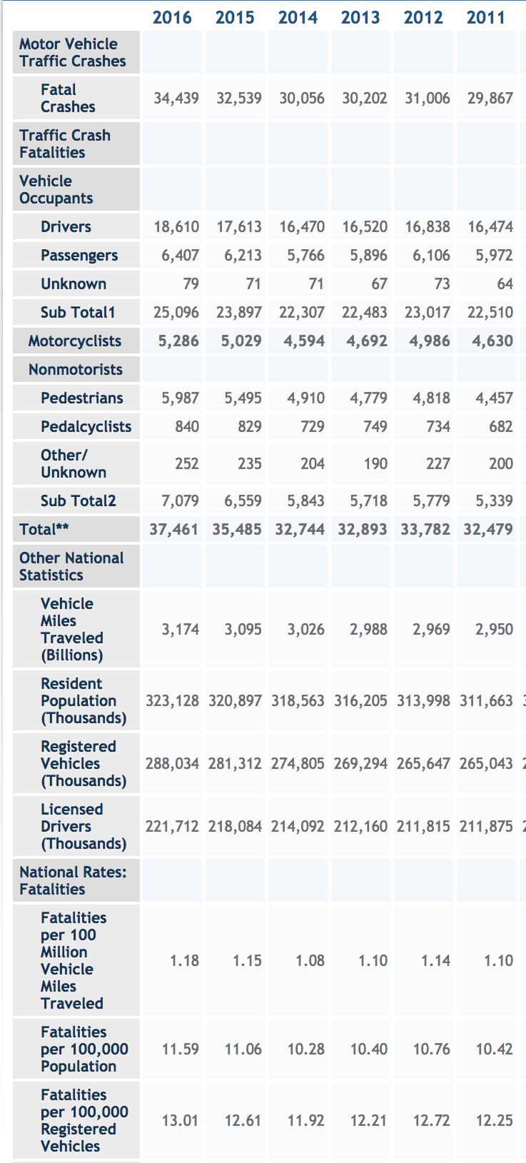
Activity 1.9 The US Department of Transportation has a program called the Fatality Analysis Reporting System. FARS has a web site which publishes data. Figure fig-bear-ride-pants1 shows a partial screen shot of their web page.
For several reasons, the table is not in tidy form.
Some of the rows serve as headers for the next several rows, but don’t contain any data. Identify several of those headers. Answer: “Motor vehicle traffic crashes”, “Traffic crash fatalities”, “Vehicle occupants”, “Non-motorists”, “Other national statistics”, “National rates: fatalities”
In tidy data, all the entries in a column should describe the same kind of quantity. You can see that all of the columns contain numbers. But the numbers are not all the same kind of quantity. Referring to the 2016 column:
- What kind of thing is the number 34,439? Answer: A number of crashes
- What kind of thing is 18,610? Answer: A number of drivers
- What kind of thing is 1.18? Answer: A rate: fatalities per 100-million miles.
In tidy data, there is a definite unit of observation that is the same kind of thing for every row. Give an example of two rows that are not the same kind of thing. Answer: For example, “Registered vehicles” and “Licensed drivers”. The first is a count of cars, the second a count of drivers.
Identify a few rows that are summaries of other rows. Such summaries are not themselves a unit of observation. Answer: “Sub Total1”, “Sub Total2”, “Total**“
Activity 1.10 Table tbl-pine-hit-pants is a re-organization and simplification of the data in Activity exr-Q01-109 about motor-vehicle related fatalities in the US. (Only part of the data is shown.)
| year | crashes | drivers | passengers | unknown | miles | resident_pop |
|---|---|---|---|---|---|---|
| 2016 | 34439 | 18610 | 6407 | 79 | 3174 | 323128 |
| 2015 | 32539 | 17666 | 6213 | 71 | 3095 | 320897 |
| 2014 | 30056 | 16470 | 5766 | 71 | 3026 | 318563 |
- In the re-organized table, what is the unit of observation? Answer: a year
- Is the re-organized table tidy data?
Answer:
Yes. (a) There is a well-defined unit of observation that is the same kind of thing for each row. (b) The values for any given variable are also the same kind of thing. For instance, drivers is the number of drivers, resident_pop is the number of people in the national population.
- For the purpose of this exercise, one of the numbers in Table tbl-pine-hit-pants has been copied with a small error. To see which it is, you’ll have to refer to Figure fig-bear-ride-pants1. Find that number and tell:
- In what year for Table tbl-pine-hit-pants does it appear? Answer: 2015
- In what variable for Table tbl-pine-hit-pants does it appear? Answer:
drivers
- The quantity presented in the variable
milesis not actually in miles. It has other units. Referring to Figure fig-bear-ride-pants1 …- What are the actual units? Answer: Billions of miles.
- Where should the information in (a) be documented? Answer: In the meta-data (codebook) for the table.
Activity 1.11 The meta-data for Table tbl-pine-hit-pants (in Activity exr-Q01-110) should include a description of each variable, its units, and what it stands for. Write such a description for the variables crashes and resident_pop. You can refer to Figure fig-bear-ride-pants1 (in Activity exr-Q01-109) for information.
Answer:
crashes– the number of motor-vehicle accidents in one year which resulted in one or more fatalities. Units: number of accidentsresident_pop– the population of the US in one year. Units: 1000s of people.
Activity 1.12 Glaucoma is a disease of the eye that is a leading cause of blindness worldwide. For those people with access to good eye health care, a diagnosis of glaucoma leads to treatment as well as monitoring of the possible progression of the disease. There are many forms of monitoring. One of them, the visual field examination, involves making measurements of light sensitivity at 54 locations arrayed across the retina. The data frame shown below (provided by the womblR R package) records the light sensitivity for one patient at each of the locations. Data from two visits – an initial visit marked 1 and a follow-up visit marked 2 which occurred 126 days after the initial visit – are contained in the data frame.
| location | day | visit | sensitivity |
|---|---|---|---|
| 1 | 0 | 1 | 25 |
| 1 | 126 | 2 | 23 |
| 2 | 0 | 1 | 25 |
| 2 | 126 | 2 | 23 |
| 3 | 0 | 1 | 24 |
| 3 | 126 | 2 | 24 |
| 4 | 0 | 1 | 25 |
| 4 | 126 | 2 | 24 |
| 5 | 0 | 1 | 26 |
| 5 | 126 | 2 | 17 |
| ... and so on for 108 rows altogether. |
- What is the unit of observation? Answer: a single location on a single visit
- Suppose a third visit was made and the new data were included in the table.
- How many columns would the revised table include? Answer: The extended table will have the same four columns.
- How many rows would the revised table include? Answer: There are 54 rows for each visit. That’s why there are 108 rows in the original table. The revised table will have 54 x 3 = 162 rows.
- Note that
dayandvisithave a very simple relationship. Construct a separate table that has all the information relatingdaytovisit. The unit of observation should be “a visit”.
Answer:
It will be a very small table. The unit of observation is “a visit” and there are only two visits, so there will be only two rows.
| visit | day |
|---|---|
| 1 | 0 |
| 2 | 126 |
Each
locationis a fixed point on the eye’s retina that can be identified by (x, y) coordinates. Here is a map showing the position of each location. Notice that location 1 has position (4, 1) and location 2 has position (5, 1). Imagine a data frame that records the position of eachlocation.- How many columns would the data frame have and what would be sensible names for them? Answer:
location,x, andy - How many rows would the data frame have? Answer: There are 54 locations so there will be 54 rows in the data frame.
- Write down the data table for positions 1, 2, 3, 4, 5, and 6.
- How many columns would the data frame have and what would be sensible names for them? Answer:
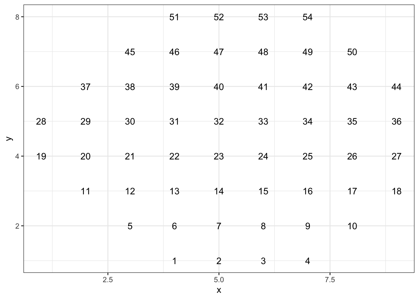
Answer:
| location | x | y |
|---|---|---|
| 1 | 4 | 1 |
| 2 | 5 | 1 |
| 3 | 6 | 1 |
| 4 | 7 | 1 |
| 5 | 3 | 2 |
| 6 | 4 | 2 |
| 7 | 5 | 2 |
| 8 | 6 | 2 |
| 9 | 7 | 2 |
| 10 | 8 | 2 |
| 11 | 2 | 3 |
| 12 | 3 | 3 |
| 13 | 4 | 3 |
| 14 | 5 | 3 |
| 15 | 6 | 3 |
| 16 | 7 | 3 |
| 17 | 8 | 3 |
| 18 | 9 | 3 |
| 19 | 1 | 4 |
| 20 | 2 | 4 |
| 21 | 3 | 4 |
| 22 | 4 | 4 |
| 23 | 5 | 4 |
| 24 | 6 | 4 |
| 25 | 7 | 4 |
| 26 | 8 | 4 |
| 27 | 9 | 4 |
| 28 | 1 | 5 |
| 29 | 2 | 5 |
| 30 | 3 | 5 |
| 31 | 4 | 5 |
| 32 | 5 | 5 |
| 33 | 6 | 5 |
| 34 | 7 | 5 |
| 35 | 8 | 5 |
| 36 | 9 | 5 |
| 37 | 2 | 6 |
| 38 | 3 | 6 |
| 39 | 4 | 6 |
| 40 | 5 | 6 |
| 41 | 6 | 6 |
| 42 | 7 | 6 |
| 43 | 8 | 6 |
| 44 | 9 | 6 |
| 45 | 3 | 7 |
| 46 | 4 | 7 |
| 47 | 5 | 7 |
| 48 | 6 | 7 |
| 49 | 7 | 7 |
| 50 | 8 | 7 |
| 51 | 4 | 8 |
| 52 | 5 | 8 |
| 53 | 6 | 8 |
| 54 | 7 | 8 |
Activity 1.13 The data table below records activity at a neighborhood car repair shop.
| mechanic | product | price | date |
|---|---|---|---|
| Anne | starter | 170.00 | 2019-01-12 |
| Beatrice | shock absorber | 78.42 | 2019-01-12 |
| Anne | alternator | 385.95 | 2019-01-12 |
| Clarisse | brake shoe | 39.50 | 2019-01-12 |
| Clarisse | brake shoe | 39.50 | 2019-01-12 |
| Beatrice | radiator hose | 17.90 | 2019-02-12 |
The codebook for a data table should describe what is the unit of observation. For the purpose of this exercise, your job is to comment on each of the following possibilities and say why or why not it is plausibly the unit of observation.
a day. Answer: There must be more to it than that, since the same date may be repeated with different values for the other variables.
a mechanic. Answer: No. The same mechanic appears multiple times, so the unit of observation is not simply a mechanic.
a car part used in a repair. Answer: Could be, for instance if every time a mechanic installs a part a new entry is added to the table describing the part, its price, the date, and the mechanic doing the work.
Enrichment topics
The preceeding text is designed to give you the essentials of data frames and how to work with them. But there is often much more to say that illuminates or extends the topics, or shows you how to perform a specialized task. These are collected at the end of each Lesson. Click on the bar to open them.
Note 1.1: Data frames in R packages
Almost all the data frames used as examples or exercises in these Lessons are stored in files provided by R software “packages” such as {LSTbook} or {mosaicData}. The data frame itself is easily accessed by a simple name, e.g., Galton. The location of the data frame is specified by the package name as a prefix followed by a pair of colons, e.g. mosaicData::Galton. A convenient feature of this system is the easy access to documentation by giving a command consisting of a question mark followed by the package-name::data-frame-name.
Note 1.2: “Tables” versus “data frames”
You may notice that the displays of data frames printed in this book are given labels such as Table tbl-galton-dataframe. It is natural to wonder why the word “table” is used sometimes and “data frame” other times.
In these Lessons we make the following distinction. A “data frame” stores values in the strict format of rows and columns described previously. Data frames are “machine readable.”
The data scientist working with data frames often seeks to create a display intended for human eyes. A “table” is one kind of display for humans. Since humans have common sense and have learned many ways to communicate with other humans, a table does not have to follow the restrictions placed on data frames. Tables are not necessarily organized in strict row-column format, can include units for numerical quantities and comments. An example is the table put together by Francis Galton (Figure fig-galton-notebook) to organize his measurements of heights.
We make the distinction between a data frame (for data storage) and a table (for communicating with humans) because many of the operations discussed in later lessons serve the purpose of transforming data frames into human-facing displays such as graphics (Lesson sec-point-plots) or tables (Enrichment topic enr-displaying-tables.)
Note 1.3: RStudio
As you get started with R, the interactive R chunks embedded in the text will suffice. On the other hand, many people prefer to use a more powerful interface, called RStudio, that allows you to edit and save files, and provides a host of other services.
There are several ways to access RStudio. For instance, it can be installed on a laptop. (Instructions for doing this are available. Use a web search to find them.) It can also be provided by a web “server.” Many colleges, universities, and other organizations have set up such servers. If you are taking a course or working in a job, your instructor or boss can tell you how to connect to such a server.
One of the nicest RStudio services is provided by posit.cloud, a “freemium” web service. The word “freemium” signals that you can use it for free, up to a point. Fortunately, that point will suffice for you to follow all of these Lessons.
- In your browser, follow this link. This will take you to
posit.cloudand, after asking you to login via Google or to set up an account, will bring you to a page that will look much like the following. (It may take a few minutes.)
- On the left half of the window, there are three “tabs” labelled “Console,” “Terminal,” and “Background Jobs.” You will be working in the “Console” tab. Click in that tab and you will see a flashing
|cursor after the>sign.
Each time you open RStudio, load the {LSTbook} package using this command at the prompt in the “console” tab.
All the R commands used in this book work exactly the same way in the embedded R chunks or in RStudio.
Note 1.4: More variable types
We are not doing full justice to the variety of possible variable types by focusing on just two type: quantitative and categorical. You should be aware that there are other kinds, for example, photographs or dates.