Imagine being transported back to June 1940. The family is in the living room sitting around the radio console waiting for it to warm up. The news today is from Europe, the surrender of the French in the face of German invasion. Follow the link, then press the play button and listen …
The spoken words from the recording are discernible despite the hiss and clicks of the background noise. The situation is similar to a conversation in a sports stadium. The crowd is loud, so the speaker has to shout. The listener filters out the noise (unless it is too loud) and recovers the shouted words.
Engineers and others make a distinction between signal and noise. The engineer aims to separate the signal from the noise. That aim applies to statistics as well.
There are many sources of noise in data. Every variable has its own story, part of which is noise from measurement errors and recording blunders. For instance, economists use national statistics, like GDP, even though the definition is arbitrary (a Hurricane can raise GDP!), and early reports are invariably corrected a few months later. Historians go back to original documents, but inevitably many of the documents have been lost or destroyed: a source of noise. Even in elections where, in principle, counting is straightforward, the voters’ intentions are measured imperfectly due to “hanging chads,” “butterfly ballots,” broken voting machines, spoiled ballots, and so on.
In this Lesson, we will take the perspective that every measurement or observation, whether quantitative or categorical, is a mixture of signal and noise. An important objective of data analysis is to identify the signal by filtering out the noise.
Consider the college-grades setting introduced in Chapter 12. The core individual measurements or observations are the student ID and the grade. Every student knows that each grade contains a noisy component caused by random factors: feeling unwell during the final exam, missed an important class meeting when you were on a varsity trip, found an unexpected extra hour for study, and so on. As well, the student ID is potentially noisy: grades get transposed between students, a record is lost in transmission to the registrar, ….
We have natural expectations that the student ID will be noiseless or, if not perfect, that errors will be vanishingly rare. To this end, colleges employ information technology (IT) specialists: engineers who design and manage computer database systems, transmission protocols, course-support software, and grade-entry user interfaces. When there is an error, the IT professionals debug the system, and make the necessary changes.
In contrast, most colleges have no quality assurance program or staff to help measure or reduce the amount of noise in a grade. But, from earlier Lessons, we now have the tools to measure noise and look for factors that introduce noise.
Noise in hiring
On several occasions, the author has testified in legal hearings as a statistical expert. In one case, the US Department of Labor audited a contractor’s records with several hundred employees and high employee turnover. The spreadsheet files led the Department to bring suit against the contractor for discriminating against Hispanics. The hiring records showed that many Hispanics applied for jobs; the company hired none. An open-and-shut case.
The lawyers for the defense asked me, the statistical expert, to review the findings from the Department of Labor. The lawyers thought they were asking me to check the arithmetic in the hiring spreadsheets. As a statistical thinker, I know that arithmetic is only part of the story; the origin of the data is critically important. So, I asked for the complete files on all applicants and hires the previous year.
The spreadsheet files and the paper job applications were in accord; there were many Hispanic applicants. But the ethnicity data on the paper job application form was not always consistent with the data on hiring spreadsheets. It turned out that whenever an applicant was hired, the contractor (per regulation) got a report on that person from the state police. The report returned by the state police had only two available race/ethnicities: white and Black. The contractor’s personnel office filled in the hired-worker spreadsheet based on the state police report. So all the Hispanic applicants who were hired had been transformed into white or Black by the state police. Noise. The Department of Labor dropped its suit. The audit had identified noise, not the signal of discrimination.
Partitioning data into signal and noise
Recall that we contemplate every observation and measurement as a combination of signal and noise.
From an isolated, individual specimen, say student sid4523 getting a grade of B+, there is no way to say what part of the B+ is signal and what part is noise. But from an extensive collection of specimens, we can potentially identify patterns across them, treating them collectively rather than as individuals.
To make a sensible partitioning of the amount of signal and the amount of noise, we need those two amounts to add up to the amount of the response variable.
We must carefully choose a method for measuring amount to ensure the above relationship holds. An example comes from chemistry: When two fluids are mixed, the volume of the mixture does not necessarily equal the sum of the volumes of the individual fluids. The same is true if we measure the amount by the number of molecules; chemical reactions can increase or decrease the number of molecules in the mixture from the sum of the number of molecules in the individual fluids. There is, however, a way to measure amount that honors the above relationship: amount measured by the mass of the fluid.
Model values as the signal
Our main tool for discovering patterns in data is modeling. For example, the pattern linking the body mass of a penguin to the sex and flipper length is:
Penguins |>model_train(mass ~ sex + flipper) |>conf_interval()
term
.lwr
.coef
.upr
(Intercept)
-5970.0
-5410
-4850.0
sexmale
268.0
348
427.0
flipper
44.1
47
49.8
Our choice of explanatory variables sets the type of signal we are looking for. In the 1940 news report from France, the signal of interest is human speech; our ears and brains automatically separate the signal from the noise. But suppose we were interested in another kind of signal, say a generator humming in the background or the dots and dashes of a spy’s Morse Code signal. We would need a different sort of filtering to pull out the generator signal, and the speech and dots and dashes (and anything else) would be noise. Identifying the dots and dashes calls for still another kind of filtering.
The same is true for the penguins. If we look for a different type of signal, say body mass as a function of the bill shape, we get utterly different coefficients:
Given the type of signal we seek to find, and the model coefficients for that type of signal, we are in a position to make a claim about what is the signal and what is the measurement in an individual penguin’s body mass. Simply evaluate the model for that penguin’s values of the explanatory variables to get the signal. What’s left over—the residuals— is the noise.
To illustrate, lets look for the sex & flipper signal in the penguins:
With_signal <- Penguins |>mutate(signal =model_values(mass ~ sex + flipper),residuals = mass - signal)
It’s time to point out something special about the residuals; there is no pattern component in the residuals. We can see that by modeling the residuals with the explanatory variables used to define the pattern:
With_signal |>model_train(residuals ~ sex + flipper) |>conf_interval()
term
.lwr
.coef
.upr
(Intercept)
-562.00
0
562.00
sexmale
-79.40
0
79.40
flipper
-2.84
0
2.84
The coefficients are zero! This means that the residuals do not show any sign of the pattern—everything about the pattern is contained in the signal!
A right triangle provides an excellent way to look at the relationship among the signal, residuals, and the response variable. We just saw that the residuals have nothing in common with the signal. This is much like the two legs of a right triangle; they point in utterly different directions!
For any triangle, any two sides add up to meet the third side. This is much like the response variable being the sum of the signal and the residuals. A right triangle has an additional property: the sum of the square lengths of the two legs gives the square length of the hypothenuse. For the penguin example, we can confirm this Pythagorean property when we use the variance to measure the “amount of” each component.
Engineers often speak of the “signal-to-noise” (SNR) ratio. In sound, this refers to the loudness of the signal compared to the loudness of the noise. For sound, the signal-to-noise ratio is often measured in decibels (dB). An SNR of 5 dB means that the signal is three times louder than the noise.
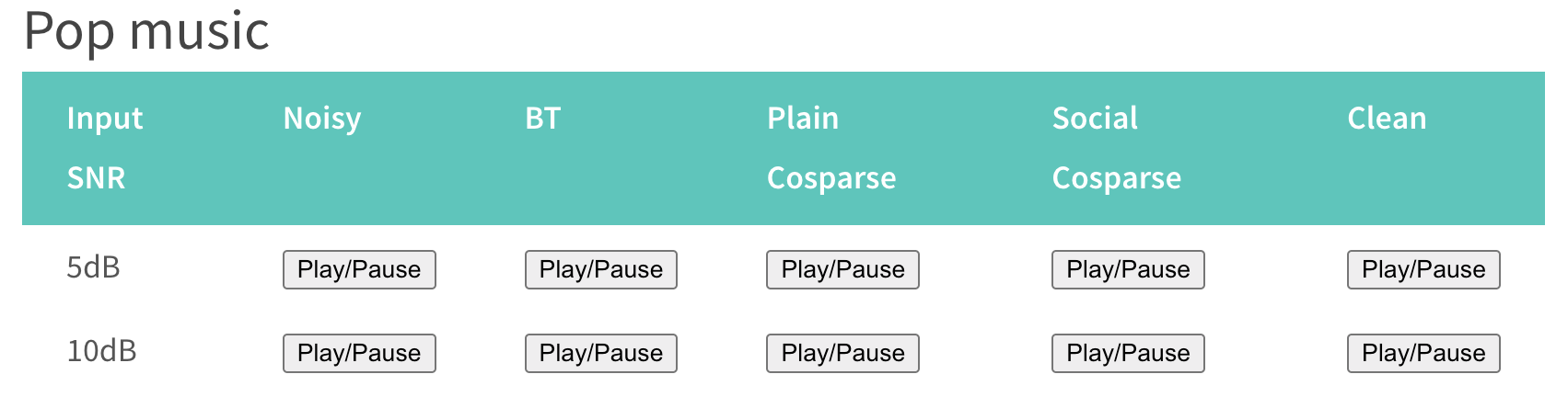
You can listen to examples of noisy music and speech at this web site, part of which looks like this:
Press the links in the “Noisy” column. The noisiest examples have an SNR of 5 dB. Press the play/pause button to hear the noisy recording, then compare it to the de-noised transmission—the signal—by pressing play/pause in the “Clean” column.
It’s easy to calculate the signal-to-noise ratio in a model pattern; divide the amount of signal by the amount of noise:
The signal is about four times larger than the noise. Converted to the engineering units of decibels, this is 6.2 dB. You can get a sense for what this means by listening to the 5 dB recordings and judging how clearly you can hear the signal.
R2 (R-squared)
Statisticians measure the signal-to-noise ratio using a measure called R2. It is equivalent to SNR, but compares the signal to the response variable instead of to the residuals. In our penguin example, mass is the response variable we chose.
R2 has an attractive property: it is always between zero and one. You can see why by considering a right triangle: a leg can never be longer than the hypothenuse, and a leg can never be shorter than zero.
We’ve already met two perspectives that statisticians take on a model: model_eval() and conf_interval(). R2 provides another perspective often (too often!) used in scientific reports. The R2() model-summarizing function does the calculations, adding in auxilliary information that we will learn how to interpret in due course.
Penguins |>model_train(mass ~ sex + flipper) |>R2()
n
k
Rsquared
F
adjR2
p
df.num
df.denom
333
2
0.806
685
0.805
0
2
330
Example: College grades from a signal-to-noise perspective
Returning to the college-grade example from Lesson 12 …. The usual GPA calculation is effectively finding a pattern in students’ grades:
Is 0.32 a large or a small R2? Researchers argue about such things. We will examine how such arguments are framed in later Lessons (especially Lesson 29).
An unconventional but, I think, helpful perspective is provided by the engineers’ way of measuring the signal-to-noise ratio: decibels. For the gradepoint ~ sid pattern, the SNR is 3.2 dB. GPA appears to be a low-fidelity, noisy signal.
A preview of things to come
We’ve pointed to the model values as the signal and the residuals as the noise. We will add another perspective on signal and noise in upcoming Lessons. The model coefficients will be treated as the signal for how the system works, the .lwr and .upr columns listed alongside the coefficients will measure the noise.
Exercises
Activity 13.1
Calculate variance of fitted values and variance of response variable. Do these give R2.
By noise we mean a variable that is utterly disconnected from any explanatory variable. We use modeling to separate signal from noise, the signal being the model values and the residuals being the noise.
To illustrate, we will use a small made-up data set, Nats and train a simple model: GDP ~ pop. Then, by evaluating the model we will get not only the model output (.output) but also the residuals (.resid).
A. The residuals are considered pure noise. As such, the explanatory variables in the model should not be able to account for the residuals at all. What is the corresponding value of R2 for .resid ~ pop?
B. Modify the tilde expression in ?lst-fit-output-pop to confirm your answer.
In communications engineering an important quantity is the power in a signal. (This is why radio stations are described technically by their output in kilowatts, a standard unit of power.) A signal-to-noise ratio is the power of the signal divided by the power of the noise.
Power is very closely related to variance. Taking the model values as the signal and the residuals as the noise, a signal-to-noise ratio can be written as the variance of the model values divided by the variance of the residuals.
TURN THIS INTO A DERIVATION OF R2 / (1 - R2)
Note 13.2: DRAFT: “Adjusted” R2
A common stage in the development of a statistical modeler is unbounded enthusiasm for using explanatory variables; the more the better!
#Nats |> mutate(r = random_terms(5)) -> foo# |>cat("This isn't working for some reason.")Nats |>model_train(GDP ~random_terms(1)) |>R2() |>select(Rsquared)
In Lesson 12 we used the word “adjustment” to refer to mathematical techniques for “holding constant” covariates.
“Adjustment” is also used in another sense in statistics. This has to do with an important modeling phenomenon: as you add explanatory variables to a model, the R2 will increase. (More precisely, it will never decrease.)
Let’s illustrate with the Children’s Respiratory Disease Study data: CRDS. We will model forced expiratory volume (FEV) using the other variables in the explanatory role.
Start with the trivial model, with no explanatory variables.
CRDS |>model_train(FEV ~1) |>R2()
n
k
Rsquared
F
adjR2
p
df.num
df.denom
654
0
0
NaN
0
NaN
0
653
As expected, since there are no explanatory variables, R2 is exactly zero.
The available explanatory variables are age, height, sex, and smoker. Modifying the chunk below, find R2 for each of these models:
FEV ~ age
FEV ~ age + height
FEV ~ age + height + sex
FEV ~ age + height + sex + smoker
CRDS |>model_train(FEV ~ age + height + sex + smoker) |>R2()
n
k
Rsquared
F
adjR2
p
df.num
df.denom
654
4
0.7753614
560.0212
0.7739769
0
4
649
Naturally, explanatory variables such as these make sense: the first three represent the size of the body, the last has well-known respiratory and cardiac impacts. But we can’t always be so sure in all settings whether the available explanatory variables genuinely explain anything. Imagine, for instance, that a variable in the data frame was just noise, having nothing to do with the response variable at all. Adding such a random variable to the model terms will nevertheless increase R2.
Let’s see this process in action. We need a new tool, one that generates random variables. We will look more deeply into such tools in Lesson 15, but for now we will use random_terms() and you’ll have to take it on faith that the values generated are random.
The random_terms() function takes one argument, an integer saying how many random variables to create. As a demonstration:
Error in draft
random_terms() isn’t working. I’ve turned the chunks off for now.
CRDS |>head() |># just a few rows, for demonstration dplyr::mutate(r =random_terms(df=2))
Admittedly, the new columns have odd-looking names—r[,1] and r[,2]—but they are ordinary columns that can be accessed via the name r. For instance:
Change the above chunk to use R2() to summarize the model rather than conf_interval(). The R2 result is close to zero, as expected considering that the r variable is random and can explain nothing.
CRDS has 654 rows. Look at R2 when we use 100 random terms rather than 4. With so many explanatory variables, R2 becomes discernably non-zero. Now try with 200 random terms, then 300. With each increase in the number of terms, R2 tends to go up, reaching close to 0.5 with 300 terms.
At the very least, this surprising result—that with enough random terms you can “explain” anything—should make you skeptical about using lots and lots of explanatory terms. But it turns out that you can take the possible randomness of explanatory variables into account, so that the use of random terms will not increase R2. One way of doing this accounting is called adjusted R2 and is reported by the R2() model summary function.
Go back and look at the adjusted R2 from your models with 100, 200, and 300 random terms. Confirm that even as R2 increases, adjusted R2 stays close to zero.
Tip 13.1
In statistics, we talk about model terms and variables. In other fields, such as physics, the preferred word is “parameters.” Physicists are taught to be distainful of models with lots of parameters, an oft-quoted phrase being, “With four parameters I can fit an elephant, and with five I can make him wiggle his trunk.”
The statistical equivalent of “wiggle his trunk” is R2 = 1. On the one hand, a model with R2 of 1 is “perfect,” it explains everything in the data.
What’s the smallest number of random terms that will lead to R2 = 1? Test this first on the Nats data frame, “explaining” the pop variable.
Try the same thing with the price variable from the Clock_auction data frame and then with the guess variable from Dowsing.
In all cases, the smallest number of random explanatory terms that will produce R2 = 1 is related to the number of rows in the data frame. Figure out what this relationship is.