9 Accounting for variation

Lesson 8 listed three foundations for statistical thinking and provided instruction on the first one:

How to measure the amount of variation in a variable

In this Lesson, we will take on two and three:

Accounting for variation in a response variable.
Measuring what remains unaccounted for.

In business, accounting keeps track of money and value: assets, receipts, expenditures, etc. Likewise, in statistics, accounting for variation is the process of keeping track of variation. At its most basic, accounting for variation splits a variable into components: those parts which can be attributed to one or more other variables and the remaining (or residual ) which cannot be so attributed.

The variable being split up is called the “response variable.” The human modeler chooses a response variable, depending on her purpose for undertaking the work. The modeler also chooses explanatory variables that may account for some of the variability in the response variable. There is almost always something left over, variation that cannot be attributed to the explanatory variables. This left-over part is called the “residual.”

To illustrate, we return to a historical statistical landmark, the data collected in the 1880s by Francis Galton on the heights of parents and their full-grown children. In that era, there was much excitement, uncertainty, and controversy about Charles Darwin’s theory of evolution.

Everyone knows that height varies from person to person. How much variation in height is there? We quantify variation using the variance. var() will do the calculation. The units of the output will be in square-inches, since height itself is measured in inches.

Learning check 9.1

Explain why var(height) has units of “square-inches” when the variable height is measured in inches.
Suppose the variance of a variable price is 144 square inches. What is the standard deviation of price? (Make sure to include the units!)
A highway traffic monitor records the speed of vehicles passing over a spot in the road. The units of speed are miles-per-hour. But the vehicles differ in speed somewhat. What will be the units of the variance of speed?

When calculating the variance of a variable, we take many pairs of values, find their difference, and square them. For instance, suppose height includes the two values 57 inches and 54 inches. The difference between them is 3 inches. The square of this difference is 9 square-inches. The variance is the average of all the different pairs of values.
The standard deviation is simply the square root of the variance. \(\sqrt{\text{144 square inches}} = \text{12 inches}\)
Since speed is measured in miles/hour, the variance of speed will have units (miles/hour)², which might equally well be written “square-miles per square hour.” Admittedly, “square hour” is a strange sounding unit, but speed and the variance of speed are different kinds of things.

Galton’s overall project was to quantify the heritability of traits (such as height) from parents to offspring. Darwin had famously measured the beaks of finches on the Galapagos Islands. Galton, in London, worked with the most readily available local species: humans. Height is easy and socially acceptable to measure, a good candidate for data collection.

Galton invented the methods we are going to use in this example.

Galton sought to divide the height variation in the children into two parts: that which could be attributed to the parents and that which remained unaccounted for, which we call the “residual.” We will start with a mathematically more straightforward project: dividing the variation in the children’s heights into that part associated with the child’s sex and the residual.

?lst-galton-mean shows how to calculate the average height for each sex using the techniques from Lesson 5. The line numbers in the code listing explain each of the components of the command.

Galton |>
1  summarize(
2    modval = mean(height),
3   .by = sex
   )

1: summarize() reduces many rows to a single row.
2: Calculate the mean of height and name the corresponding variable in the output modval.
3: Break down the calculation in (2) group by group.

sex
modval


M
69.23

F
64.11

sex	modval
M	69.23
F	64.11

To see the results of the command, run it!

Note that the output has one row for each sex. As always, the output from summarize is set by the arguments to the function. Here, there will be two variables in the output: sex and the mean height for each sex, which we’re calling modval, short for model value.

This simple report indicates that the sexes differ, on average, by about 5 inches in height. But this report offers no insight into how much of the person-to-person variation in height is attributable to sex. For that, we need to look at the group averages in the context of the variation of individuals. That is, instead of computing the model value for each sex, we will compute it for each specimen using mutate(). This is simple, since all F specimens will have a model value of 64.1 inches, while the M specimens all have a model value of 69.2 inches. However, anticipating what will come later in this Lesson, we will do the calculation using mutate().

Listing 9.1

Note: To save space on the screen, Listing 9.1 is written to show only a handful of the 898 rows that would otherwise be in the output.

Listing 9.2 repeats the above calculation, but summarizes to show the variance of height and the variance of the model values.

Listing 9.2

The output shows that the variability in the model values of height, is about half the variability in the height itself. This is the the answer to (2) from the introduction to this Lesson; sex accounts for about half of the variation in height.

Item (3) in the introduction was about measuring what remains unexplained. This “unexplained” part of height is called the residual from the model values. The residual is easy to calculate. Listing 9.3 calculates the residuals from the simple model that accounts for height by sex.

Listing 9.3

It’s essential to note from the output of Listing 9.3 that the variance in the response variable (height) is exactly the sum of the the variance of the model values and the variance of the residuals. In other words, the variance in the response variable is perfectly split into two parts:

the part accounted for by the explanatory variable and
the part that remains unaccounted for.

Learning check 9.2

Listing 9.3 shows how to calculate the residual for each specimen: subtract the model value from the value of the response variable. Let’s look at the values of the residuals from the model of height versus sex.

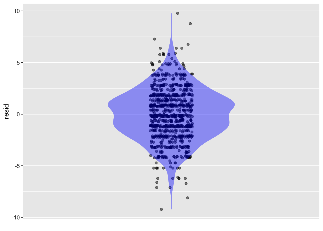
Which line of Listing 9.9 finds the residual for each of the specimens?
Some residuals are positive and some negative. Explain how a residual can be negative.

If the model value is larger than the response variable, the residual will be negative. Similarly, if the model value is less than the response variable, the residual is positive.

Learning check 9.3

Since Lesson [-@sec--variation-and-distribution] we have used the variance as the prefered way to measure the amount of variation. The advantage of the variance is that it perfectly partitions variation in the response variable into two parts: (i) variation in the model values and (ii) variation in the residuals.

The following chunk demonstrates the perfect partitioning: Run it!

Listing 9.5

Modify the above chunk to model the age of a mother (mage) from the Births2022 data frame by the mother’s education level (meduc). Is the variation in mage perfectly partitioned between the model values and the residuals?

In addition to replacing Galton with Births2022, you will need to replace the explanatory variable sex with meduc. Similarly, replace height with mage.

Some people prefer to use the standard deviation (sd()) to measure variation. Modify the above chunk, replacing var() with sd(). Looking at the results, does the standard deviation perfectly partition the response variable into model values and residuals?

The variance of any response variable will always be split perfectly between the variance of the model values and the variance of the residuals. This is a mathematical fact that stems from the same phenomenon as in the Pythagorean Theorem.
The standard deviation of the response is not split perfectly by the standard deviation of the model values and the standard deviation of the residuals.

Numerical explanatory variables

The previous section used the categorical variable sex as the explanatory variable. Galton’s interest, however, was in the relationship between children’s and parents’ height.

sex is a categorical explanatory variable. Using mutate(..., .by = sex) is a good method of handling categorical explanatory variables. However, this does not work for quantitative explanatory variables. The reason is that .by translates a quantitative variable into a categorical one, with a result for each unique quantitative value. It’s trivial to substitute the height of the mother or father in place of sex in the method introduced in the previous section. However, as we shall see, the results are not satisfactory. Galton’s key discovery was the proper method for relating two quantitative variables such as height and mother.

First, let’s try simply substituting in mother as the explanatory variable and using mean() to create the model values. Then, use point_plot() to show the model values as a function of mother.

Listing 9.6

The last line of Listing 9.6 connects adjacent points with lines. It’s hard to see any pattern in the model values.

It is common sense that the model linking mothers’ heights to children’s height should be smooth, not the jagged pattern seen in Listing 9.6. The source of the jaggedness is the use of .by = mother in mutate(modval = mean(height), .by = mother). There is nothing in .by = mother to enforce the idea that the model value for mid-height mothers should be in-between the model values for short and for tall mothers.

The solution to the problem of jagged model values is to avoid the absolute splitting into non-overlapping groups by mother’s height. Instead, we want to find a smooth relationship. Galton invented the method for accomplishing this. A modern form of his method is provided by the model_values() function., which we shall use to construct Model3.

Listing 9.7

Notice that the .by = mother step has been entirely removed. Notice also that model_values() uses the same kind of tilde expression as we have employed when plotting. The response variable is listed on the left of the , the explanatory variable on the right side. In other words, we are modeling the child’s height as a function of mother’s height.

As always, modeling splits the variance of the response variable into two parts, one associated with the explanatory variable and the other holding what’s left over: the residual. Here’s the split for Model3 which uses mother as an explanatory variable:

Listing 9.8

The mother’s height doesn’t account for much of the variation in the children’s heights.

Learning check 9.4

The model_values() approach to modeling works for both quantitative and categorical explanatory variables. For convenience, you can annotate point_plot() to show the model along with the raw data. Try it:

Listing 9.9

From the graph, estimate the largest positive residual among the females.

The model value for females is about 64 inches. The tallest female is 71 inches. This makes the largest residual 71 - 64 = 5 inches.

Change the code in the chunk to show the model height ~ mother. Find a point that has a large negative residual from this model.

Multiple explanatory variables

The models we work with in these Lessons always have exactly one response variable. But models can have any number of explanatory variables.

Note that the idea of “response” and “explanatory” variables refers to a model and are not at all intrinsic to a bare data frame. A data frame can contain many variables, any of which can be used as explanatory variables. The choice of response variable depends on the modeler’s goals.

Whatever the number of explanatory variables and however many levels a categorical explanatory variable has the model splits the variance of the response into two complementary pieces: the variance accounted for by the explanatory variables and the part not accounted for, that is, the residual variance.

Many statistical terms mean something different in statistical than in everyday use. “Residual” is a pleasant exception: the statistical meaning is closely matched by its everyday dictionary definition.

To illustrate, here is a sequence of models of height with different numbers of explanatory variables.

Number of explanatory variables	tilde expression	`var(resid)`
0	`height ~ 1`
1	`height ~ sex`
2	`height ~ sex + mother`
3	`height ~ sex + mother + father`

Plugging each of these number

Galton |>
  mutate(modval =
           model_values(
             ..tilde.expression.here.
             ),
         resid = height - modval) |>
  summarize(var(height), var(modval), var(resid))

Three explanatory variables

YOU WERE HERE: Perhaps convert this to an interactive

Galton |>
  mutate(modval = 
           model_values(height ~ sex + mother + father),
         resid = height - modval) |>
  summarize(var(height), var(modval), var(resid))

var(height)
var(modval)
var(resid)


12.8373
8.211706
4.625599

var(height)	var(modval)	var(resid)
12.8373	8.211706	4.625599

Two explanatory variables

Galton |>
  mutate(modval = 
           model_values(height ~ sex + mother),
         resid = height - modval) |>
  summarize(var(height), var(modval), var(resid))

var(height)
var(modval)
var(resid)


12.8373
7.212022
5.625283

var(height)	var(modval)	var(resid)
12.8373	7.212022	5.625283

One explanatory variable

Galton |>
  mutate(modval = model_values(height ~ sex),
         resid = height - modval) |>
  summarize(var(height), var(modval), var(resid))

var(height)
var(modval)
var(resid)


12.8373
6.549134
6.288171

var(height)	var(modval)	var(resid)
12.8373	6.549134	6.288171

Zero explanatory variables

Galton |>
  mutate(modval = model_values(height ~ 1),
         resid = height - modval) |>
  summarize(var(height), var(modval), var(resid))

var(height)
var(modval)
var(resid)


12.8373
0
12.8373

var(height)	var(modval)	var(resid)
12.8373	0	12.8373

Comparing models with R²

When selecting explanatory variables, comparing two or more different models sharing the same response variable is often helpful: a simple model and a model that adds one or more explanatory variables to the simple model. The model with no explanatory variables, is always the simplest possible model. For example, in Section 9.2, the model height ~ 1 is the simplest. Compared to the simplest model, the model height ~ sex has one additional explanatory variable, sex. Similarly, height ~ sex + mother has one additional explanatory variable compared to height ~ sex, and height ~ sex + mother + father adds in still another explanatory variable.

The simpler model is said to be “nested in” the more extensive model, analogous to a series of Matroshka dolls. A simple measure of how much of the response variance is accounted for by the explanatory variables is the ratio of the variance of the model values divided by the variance of the response variable itself. This ratio is called “R²”, pronounced “R-squared.”

A sequence of five nested Matroshka dolls. Each smaller doll fits inside a larger one.

For instance, R^2 for the model height ~ sex + mother is \[\text{R}^2 = \frac{7.21}{12.84} = 0.56\] By comparison, R^2 for the simpler model, height ~ sex, is slightly smaller:

R² is also known as the “coefficient of determination,” a little-used term we shall avoid. Still, it’s worth noting the attitude behind the term; it quantifies the extent to which the response variable is “determined” by the explanatory variables.

\[\text{R}^2 = \frac{6.55}{12.84} = 0.51\] For all models, \(0 \leq\) R² \(\leq 1\). It is tempting to believe that the “best” model in a set of nested models is the one with the highest R², but statistical thinkers understand that “best” ought to depend on the purpose for which the model is being built. This matter will be a major theme in the remaining Lessons.

Instructor Note: Strictly speaking, “all” should be qualified to mean “linear least-squares models with an intercept term.”

Exercises

Exercise 9.1 The data frame LSTbook::Gilbert records 1641 shifts at a VA hospital. (For the story behind the data, give the command ?Gilbert.) Whether or not a patient died during a shift is indicated by the variable death. The variable gilbert marks whether or not nurse Kristen Gilbert was on duty during the shift.

A. Are the variables numerical or categorical?

B. The data were used as evidence during Gilbert’s trial for murder. The data can be reduced to a compact form by data wrangling:

LSTbook::Gilbert |> 
  summarize(count = n(), .by = c(death, gilbert))

death
gilbert
count


no
not
1027

yes
not
357

no
on_duty
157

yes
on_duty
100

death	gilbert	count
no	not	1027
yes	not	357
no	on_duty	157
yes	on_duty	100

Calculate the proportion of times a death occurred when Gilbert was on duty, and the proportion of time when Gilbert was not on duty. Does the shift evidence support the claim that Gilbert was a contributing factor to the deaths.

C. In the Lessons, we will mainly use regression modeling rather than wrangling as a data-reduction technique. In the trial, the relevant question was whether Gilbert was a factor in the deaths. Express this question as a tilde expression involving the variables death and gilbert.

D. The response variable in your tilde expression from (C) is categorical. Regression modeling requires a numerical response variable. Use mutate() and zero_one() to transform the variable death from categorical form to a numerical form that has a value 1 when Gilbert was on duty and 0 otherwise. This will become the response variable for the regression: death ~ gilbert.

E. Carry out the regression using model_train(). Look at the coefficients from the fitted model with conf_interval(); these are in .coef column. Explain how the coefficients correspond to the proportions you calculated in (B).

id=Q09-101

Exercise 9.2

DRAFT: Which variables could be used as response variables?

id=Q09-102

Exercise 9.3

DRAFT: Do a nested model approach with Anthro_F and R²

id=Q09-103

Exercise 9.4

DRAFT: Show that the sum of squares and mean square for modeling using the median is larger than for the mean.

id=Q09-104

Exercise 9.5

DRAFT: Simple calculation of \(R^2\).

id=Q09-105

Exercise 9.6

id=Q09-106

Numerical explanatory variables

Multiple explanatory variables

Comparing models with R2

Exercises

Comparing models with R²