28 Bayesian competition between hypotheses
\[\newcommand{\Ptest}{\mathbb{P}} \newcommand{\Ntest}{\mathbb{N}} \newcommand{\Sick}{\cal S} \newcommand{\Healthy}{\cal H} \newcommand{\given}{\ |\!\!|\ }\]
The test of a first-rate intelligence is the ability to hold two opposed ideas in the mind at the same time, and still retain the ability to function. – F. Scott Fitzgerald, 1936
Our actions are guided by what we know about the state of things and the mechanisms that shape that state. Experience shows, however, that sometimes our so-called “knowledge” is only approximate or even dead wrong. Acknowledging this situation, in these Lessons we have avoided the word “knowledge” in favor of “hypothesis.”
“To entertain a hypothesis” is to express a willingness to take that hypothesis into consideration as we try to make sense of the world. We can entertain more than one hypothesis about any given situation, but frequently we give more credence to one hypothesis than to another. It is as if multiple hypotheses are competing for credibility as explanations for the events seen in the world.
Bayesian inference provides a framework for calculating how we should balance the credence we give different hypotheses in the light of accumulating data. It does this quantitatively, using the language of probability to represent what in English we call variously credibility, credence, belief, faith, credit, credulity, confidence, certitude, and so on .
In this Lesson, we introduce Bayesian inference in a simple context: a competition between two opposing hypotheses. Later, in Lesson 29, we will use the Bayesian framework to illuminate two other widely-used forms of statistical inference: null hypothesis testing and the Neyman-Pearson framework.
Two hypotheses in the light of data
Bayesian inference is applicable to many situations. We will use the familiar one of health. In particular, imagine a disease or condition that a person might or might not have, for instance, COVID or breast cancer. The two competing hypotheses are that you are sick or you are healthy. Medical diagnosis generally involves more than two hypotheses: a range of possible illnesses or conditions. But, in this introduction, we will keep things simple.
We will denote the two hypotheses—sick or healthy—as \(\Sick\) and \(\Healthy\).
A medical test (such as mammography or an at-home COVID test) is a common source of data to inform the relative credibility of the two hypotheses. Many such medical tests are arranged to produce a binary outcome: either a positive (\(\Ptest\)) or a negative (\(\Ntest\)) result. By convention, a positive test result points toward the subject of the test being sick and a negative tests points toward being healthy.
The test produces a definite observable result that can have one, and only one, outcome: \(\Ptest\) or \(\Ntest\). In contrast, \(\Sick\) and \(\Healthy\) are hypotheses that are competing for credulity . We can entertain both hypotheses at the same time. A typical situation in medical testing is that a \(\Ptest\) results triggers additional tests, for instance a biopsy of tissue. It’s often the case that the additional tests contradict the original test. A biopsy performed after a \(\Ptest\) often turns out to be negative. In many situations, “often” means “the large majority of the time.”
Confusing an observable result with a hypotheses leads to faulty reasoning. The fault is not necessarily obvious. For example, it seems reasonable to say that “a positive test implies that the patient is sick.” In the formalism of logic, this could be written \(\Sick\impliedby\Ptest\). One clue that this simple reasoning is wrong is that \(\Ptest\) and \(\Sick\) are different kinds of things: one is an observable and the other is a hypothesis.
Another clue that \(\Sick\impliedby\Ptest\) is fallacious comes from causal reasoning. A positive test does not cause you to become sick. To the contrary, sickness creates the physical or biochemical conditions cause the test to come out \(\Ptest\). And we know that \(\Ptest\)s can occur even among the healthy. (These cases are called “false positives”.)
Bayesian inference improves on the iffy logic of implication when considering which of two hypotheses—\(\Sick\) or \(\Healthy\)—is to be preferred based on the observables.
Probability and likelihood
One step toward a better form of reasoning is to replace the hard certainty of logical implication with something softer: probability and likelihood. Instead of \(\Ptest \impliedby \Sick\), it’s more realistic to say that the likelihood of \(\Ptest\) is high when the patient is \(\Sick\). Or, in the notation of likelihood :
Recall from Lesson 16 that a likelihood is the probability of observing a particular outcome—\(\Ptest\) here—in a world where a hypothesis—\(\Sick\) here—is true.
\[p(\Ptest\given\Sick)\ \text{ is high, say, 0.9.} \tag{28.1}\]
If the test is any good, a similar likelihood statement applies to healthy people and their test outcomes:
\[p(\Ntest\given\Healthy)\ \text{is also high, say, 0.9.} \tag{28.2}\]
These two likelihood statements represent well, for instance, the situation with mammography to detect breast cancer in women. Unfortunately, although both statements are correct, neither is directly relevant to a woman or her doctor interpreting a test result. Instead, the appropriate interpretation of \(\Ptest\) comes from the answer to this question:
Suppose your test result is \(\Ptest\). To what extent should you believe that you are \(\Sick\)? That is, how much credence should you give the \(\Sick\) hypothesis, as opposed to the competing hypothesis \(\Healthy\)?
It’s reasonable to quantify the extent of credibility or belief in terms of probability. Doing this, the above question becomes an of finding \(p(\Sick\given\Ptest)\). Also relevant, at least for the woman getting a \(\Ntest\) result is the probability \(p(\Healthy\given\Ntest)\).
Using probabilities to encode the extent of creditability has the benefit that we can compute some things from others. For example, from \(p(\Sick\given\Ptest)\) we can easily calculate \(p(\Healthy\given\Ptest)\): the relationship is \[p(\Healthy\given\Ptest) = 1 - p(\Sick\given\Ptest) .\] Notice that both of these probabilities have the observation \(\Ptest\) as the given. Similarly, \(p(\Sick\given\Ntest) = 1 - p(\Healthy\given\Ntest)\). Both of these have the observation \(\Ntest\) as given.
Now consider the likelihoods as expressed in Statements 28.1 and 28.2. There is no valid calculation on the likelihoods that is similar to the probability calculations in the previous paragraph. \(1-p(\Ptest\given\Sick)\) is not necessarily even close to \(p(\Ptest\given\Healthy)\). To see why, consider the metaphor about planets made in Section 27.3. Planet \(\Sick\) is where \(p(\Ptest\given\Sick)\) can be tabulated, but \(p(\Ptest\given\Healthy)\) is about the conditions on Planet \(\Healthy\). Being on different planets, the two probabilities have no simple relationship. Let’s emphasize this.
- In \(p(\Ptest\given\Sick)\), we stipulate that you are \(\Sick\) and ask how likely would be a \(\Ptest\) outcome under the \(\Sick\) condition.
- In \(p(\Sick\given\Ptest)\), we know the observed test outcome is \(\Ptest\) and we want to express how strongly we should believe in hypothesis \(\Sick\).
To avoid confusing (i) and (ii), we will write (i) using a different notation, one that emphasizes that we are talking about a \(\cal L}\text{ikelihood}\). Instead of \(p(\Ptest\given\Sick)\), we will write \({\cal L}_\Sick(\Ptest)\). Read this as “the likelihood on planet \(\Sick\) of observing a \(\Ptest\) result. This can also be stated (with greater dignity) in either of these ways:”The likelihood under the assumption of \(\Sick\), of observing a \(\Ptest\) result,” or “stipulating that the patient is \(\Sick\), the likelihood of observing \(\Ptest\).” \(p(\Ptest\given\Sick)\) and \({\cal L}_\Sick(\Ptest)\) are just two names for the same quantity, but \({\cal L}_\Sick(\Ptest)\) is a reminder that this quantity is a likelihood.
Prior and posterior probability
Recall the story up to this point: You go to the doctor’s office and are going to get a test. It matters greatly why you are going. Is it just for a scheduled check-up, or are you feeling symptoms or seeing signs of illness?
In the language of probability, this why is summarized by what’s called a “**prior probability, which we can write \(p(\Sick)\). It’s called a “prior” because it’s relevant before* you take the test. If you are going to the doctor for a regular check-up, the prior probability is small, no more than the prevalence of the sickness in the population you are a part of. However, if you are going because of signs or symptoms, the prior probability is larger, although not necessarily large in absolute terms.
Your objective in going to the doctor and getting the test is to get more information about whether you might be sick. We express this as a “posterior probability,” that is, your revised probability of being \(\Sick\) once you know the test result.
The point of Bayesian reasoning is to use new observations to turn a prior probability into a posterior probability. That is, the new observations allow you to update your previous idea of the probability of being \(\Sick\) based on the new information.
There is a formula for calculating the posterior probability. The formula can be written most simply if both the prior and the posterior are represented as odds rather than as probability. Recall that if the probability of some outcome is \(p(outcome)\), then the odds of that outcome is \[\text{Odds}(\text{outcome}) \equiv \frac{p(\text{outcome})}{1 - p(\text{outcome})} .\]
Learning check 28.1
REVIEW the transformation from probabilities to odds and back.
odds = p/(1-p)
p = odds/(1+odds)
THEN SHOW HOW RELATIVE strengths of belief can be formatted as odds and then transformed to the probability of one of the hypotheses (with the probability of the other being the complement).
For instance, a possible Bayesian statement about \(\Sick\) and \(\Healthy\) goes like this, “In the relevant instance, my belief in \(\Sick\) is at a level of 7, while my belief in \(\Healthy\) is only 5.” But what are the units of 7 and of 5? Perhaps surprisingly, it doesn’t matter. The odds for \(\Sick\) will be 7/5. Correspondingly, the prior odds for \(\Healthy\) will be 5/7.
For future reference, here is the formula for the posterior odds. We present and use it here, and will explain its origins in the next sections of this Lesson. It is called Bayes’ Rule .
\[\text{posterior odds of }\Sick = \frac{\cal{L}_\Sick(\text{test result})}{\cal{L}_\Healthy(\text{test result})}\ \times \text{prior odds of }\Sick \tag{28.3}\]
Formula 28.3 involves two hypotheses and one observed test result. Each of the hypotheses corresponds to the likelihood of the observed test result. The relative credit we give the hypotheses is measured by the odds. If the odds of \(\Sick\) are greater than 1, \(\Sick\) is preferred. If the odds of \(\Sick\) are less than 1, \(\Healthy\) is preferred. The prior odds apply before the test result is observed, the posterior odds apply after the test result is known.
The two hypotheses—\(\Sick\) or \(\Healthy\)—are competing with one another. The quantitative representation of this competition is called the Likelihood ratio .
\[\textbf{likelihood ratio:}\ $\frac{\cal{L}_\Sick(\text{test result})}{\cal{L}_\Healthy(\text{test result})} .\]
Let’s illustrate using the situation of a 50-year old woman getting a regularly scheduled mammogram. Before the test, in other words, prior to the test, her probability of having breast cancer is low, say 1%. Or, reframed as odds, 1/99.
It turns out that the outcome of the test is \(\Ptest\). Based on this, the formula lets us calculate the posterior odds. Since the test result is \(\Ptest\), the relevant likelihoods are \(\cal L_\Sick(\Ptest)\) and \(\cal L_\Healthy(\Ptest)\). Referring to 28.1 and 28.2 in the previous section, these are
\[\cal L_\Sick(\Ptest) = 0.90 \ \text{and}\ \ \cal L_\Healthy(\Ptest) = 0.10 .\]
Consequently the likelihood ratio is
\[\frac{\cal L_\Sick(\Ptest)}{\cal L_\Healthy(\Ptest)} = \frac{0.90}{0.10} = 9 .\]
Learning check 28.2
Statement 28.1 describes the likelihood of observing \(\Ptest\) under the hypothesis that the patient is \(\Sick\): \(\cal L_\Sick(\Ptest)\). We said that for mammography, this likelihood is about 0.9.
Similarly, statement 28.2, about \(\cal L_\Healthy(\Ntest)\) is the likelihood of observing \(\Ntest\) under a different hypothesis, that the patient is \(\Health\). Coincidentally, for mammography, this, too, is about 0.9.
How do we know that \(\cal L_\Healthy(\Ptest)\) is, accordingly, about 0.1?
An observation of \(\Ptest\) is the alternative to an observation of \(\Ntest\), consequently, the probability of \(\Ptest\) (under the hypothesis \(\Healthy\)) is the complement of the probability of \(\Ntest\), that is \(1 - \cal L_\Healthy(\Ntest) = 1 - 0.9 = 0.1\).
The formula says to find the posterior odds by multiplying the prior odds by the likelihood ratio. The prior odds were 1/99, so the posterior odds are \(9/99 = 0.091\). This is in the format of odds, but most people would prefer to reformat it as a probability. This is easily done: the posterior probability of \(\Sick\) is \(\frac{0.091}{1 + 0.091} = 0.083\).
Perhaps this is surprising to you. The posterior probability is small, even though the woman had a \(\Ptest\) result. This surprise illustrates why it is so important to understand Bayesian calculations.
Learning check 28.3
DRAFT: Applying the Bayes formula.
We used a prior probability of 0.01 for a 50-year-old woman who goes for a regularly scheduled mammogram. Suppose, however, that a second woman gets a mammogram because of a lump in her breast. Given what we know about lumps and breast cancer, this second woman will have a higher prior, let us say, 0.05. Given a \(\Ptest\) result from the mammogram, what is the posterior probability of \(\Sick\).
Or, prior probability for a sports team that was no good last year, but has had an excellent first three games.
If the prior probability for the second woman is 0.05, then her prior odds are \(5/95 = 0.053\). The likelihood ratio, however, is the same for both women: 9. That’s because the test is not affected by the women’s priors, it is about the physics of X-rays passing through different kinds of tissue. Multiplying the prior odds by the likelihood gives 0.47, a much higher posterior than the 0.083 we calculated for the woman who went at the regularly scheduled time.
Perhaps this is obvious, but it’s still worth pointing out. The woman with the lump will not do better by waiting for the regularly scheduled time for her mammogram. Even if she does, the prior will be based on the lump.
Basis for Bayes’ Rule
To see where Bayes’ Rule comes from, let’s look back into the process of development of the medical test that gives our observable, either \(\Ptest\) or \(\Ntest\).
Test developers start with an idea about a physically detectable condition that can indicate the presence of the disease of interest. For example, observations that cancerous lumps are denser than other tissue probably lie at the origins of the use of x-rays in the mammography test. Similarly, at-home COVID tests detect fragments of proteins encoded by the virus’s genetic sequence. In other words, there is some physical or biochemical science behind the test. But this is not the only science.
The test developers also carry out a trial to establish the performance of the test. One part of doing this is to construct a group of people who are known to have the disease. Each of these people is then given the test in question and the results tabulated to find the fraction of people in the group who got a \(\Ptest\) result. This fraction is called the test’s sensitivity Estimating sensitivity is not necessarily quick or easy; it may require use of a more expensive or invasive test to confirm the presence of the disease, or even waiting until the disease becomes manifest in other ways and constructing the \(\Sick\) group retrospectively.
At the same time, the test developers assemble a group of people known to be \(\Healthy\). The test is administered to each person in this group and the fraction who got a \(\Ntest\) result is tabulated. This is called the specificity of the test.
Figure 28.2 shows schematically the people in the \(\Sick\) group alongside the people in the \(\Healthy\) group. The large majority of the people in \(\Sick\) tested \(\Ptest\): 90% in this illustration. Similarly, the large majority of people in \(\Healthy\) tested \(\Ntest\): 80% in this illustration.

The sensitivity and specificity are both likelihoods. Sensitivity is the probability of a \(\Ptest\) outcome given that the persion is \(\Sick\). Specificity is the probability of a \(\Ntest\) outcome given that the person in \(\Healthy\). To use the planet metaphor of Lesson 27, the specificity is calculated on a planet where everyone is \(\Healthy\). The sensitivity is calculated on a different planet, one where everyone is \(\Sick\).
Figure 28.2 shows schematically the people in the \(\Sick\) group alongside the people in the \(\Healthy\) group. The large majority of the people in \(\Sick\) tested \(\Ptest\): 90% in this illustration. Similarly, the large majority of people in \(\Healthy\) tested \(\Ntest\): 80% in this illustration.


Now turn to the use of the test among people who might be sick or might be healthy. We don’t know the status of any individual person, but we do have some information about the population as a whole: the fraction of the population who have the disease. This fraction is called the prevalence of the disease and is known from demographic and medical records.
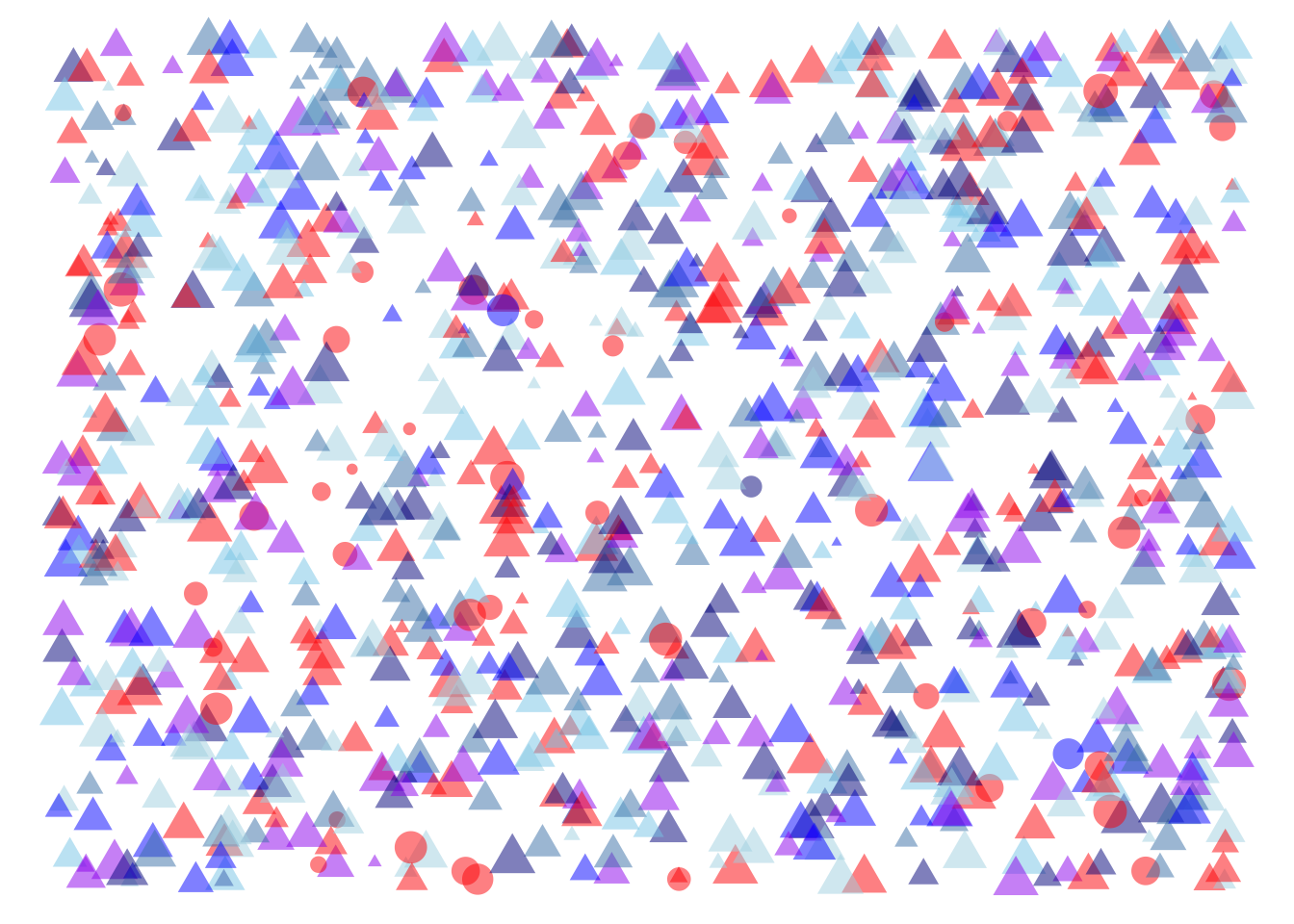
For the sake of illustration, Figure 28.3 shows a simulated population of 1000 people with a prevalence of 5%. That is, fifty dots are circles, the rest triangles. Each of the 1000 simulated people were given the test, with the result shown in color (red is \(\Ptest\)).
The nature of a simulation is that we know all the salient details about the individual people, in particular their health status and their test result. This makes it easy to calculate the posterior probability, that is, the fraction of people with a \(\Ptest\) who are actually \(\Sick\). To illustrate, we will move people into a quadrant of the field depending on their status:
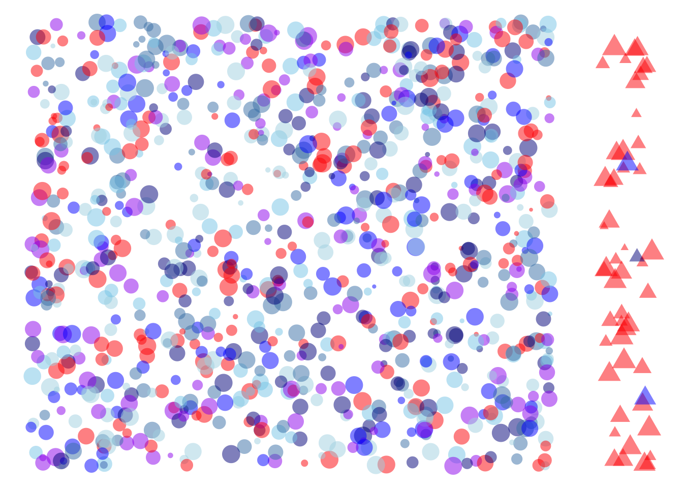
The same people as in Figure 28.3 repositioned according the their health status and test result.
Figure 28.4(a) illustrates the prevalence of the disease, that is, the fraction of people with the disease. This is the fraction of people moved to the right side of the field, all of whom are triangles. Almost all of the \(\Sick\) people had a \(\Ptest\) result, reflecting a test sensitivity of 90%.
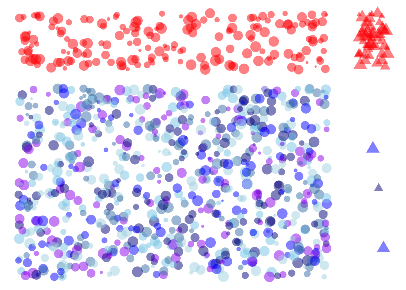
Figure 28.4(b) further divides the field. All the people with a \(\Ptest\) result have been moved to the top of the field. Altogether there are four clusters of people. On the bottom left are the healthy people who got an appropriate \(\Ntest\) result. On the top right are the \(\Sick\) people who also got the appropriate test result: \(\Ptest\). On the bottom right and top left are people who were mis-classified by the test.
The group on the bottom right is \(\Sick\) people with a \(\Ntest\) result. These test results are called false negatives —“false” because the test gave the wrong result, “negative” because that result was \(\Ntest\).
Similarly, the group on the top left is mis-classified. All of them are \(\Healthy\), but nonetheless they received a \(\Ptest\) result. Such results are called false positives . Again, “false” indicates that the test result was wrong, “positive” that the result was \(\Ptest\).
Now we are in a position to calculate, simply by counting, the posterior probability. That is, the probability that a person with a \(\Ptest\) test resuult is actually \(\Sick\).
| sick | test | n |
|---|---|---|
| H | N | 763 |
| H | P | 185 |
| S | N | 3 |
| S | P | 49 |
If you take the time to count, in Figure 28.4 you will find 185 people who are \(\Healthy\) but erroneously have a \(\Ptest\) result. There are 49 people who are \(\Sick\) and were correct given a \(\Ptest\) result. Thus, the odds of being \(\Sick\) given a \(\Ptest\) result are 49/185 = 0.26, which is equivalent to probability of about 20%.
Let’s compare the counting result to the result from Bayes’ Rule (Equation 28.3).
- Since the prevalence is 5%, the prior odds are 5/95.
- The likelihood of a \(\Ptest\) result for \(\Sick\) people is exactly what the sensitivity measures: 90%.
- The likelihood of a \(\Ntest\) result for \(\Healthy\) people is one minus the specificity: 1 - 80% = 20%.
Putting these three numbers together using @eq_bayes-rule-odds gives the posterior odds:
\[\underbrace{\frac{90\%}{20\%}}_\text{Likelihood ratio}\ \ \ \times\ \ \underbrace{\frac{5}{95}}_\text{prior odds} = \underbrace{\ 0.24\ }_\text{posterior odds}\]
The result from Bayes’ Rule differs very little from the posterior odds we found by simulation counting. The difference is due to sampling variation; our sample from the simulation had size \(n=1000\). But had we used a much larger sample, the results would converge on the result from Bayes’ Rule.
Exercises
Exercise 28.1
Exercise 28.2
A common mis-interpretation of a confidence interval is that it describes a probability distribution for the “true value” of a coefficient. There are two aspects to this fallacy. The first is philosophical: the ambiguity of the idea of a “true value.” A coefficient reflects not just the data but the covariates we choose to include when modeling the data. Statistical thinkers strive to pick covariates in a way that matches their purpose for analyzing the data, but there can be multiple such purposes. And, as we’ll see in Lesson 25, even for a given purpose the best choice depends on which DAG one takes to model the system.
A more basic aspect to the fallacy is numerical. We can demonstrate it by constructing a simulation where it’s trivial to say what is the “true value” of a coefficient. For the demonstration, we’ll use sim_02 modeled as y ~ x + a, but we could use any other simulation or model specification.
Here’s a confidence interval from a sample of size 100 from sim_02.
set.seed(1014)
sim_02 |>take_sample(n = 100) |>
  model_train(y ~ x + a) |>
  conf_interval() |>
filter(term == "x")| term | .lwr | .coef | .upr |
|---|---|---|---|
| x | 2.912935 | 3.107641 | 3.302346 |
Now conduct 250 trials in which we sample new data and find the x coefficient.
set.seed(392)
Trials <-
  sim_02 |>take_sample(n = 100) |>
  model_train(y ~ x + a) |>
  conf_interval() |>
  filter(term == "x") |>
  trials(250)
We will plot the coefficients from the 500 trials along with the coefficient and the confidence interval from the reference sample:
Trials |>
  point_plot(.coef ~ 1, annot = "violin") |>
  gf_point(3.11 ~ 1, color = "red") |>
  gf_errorbar(2.91 + 3.30 ~ 1, color = "red")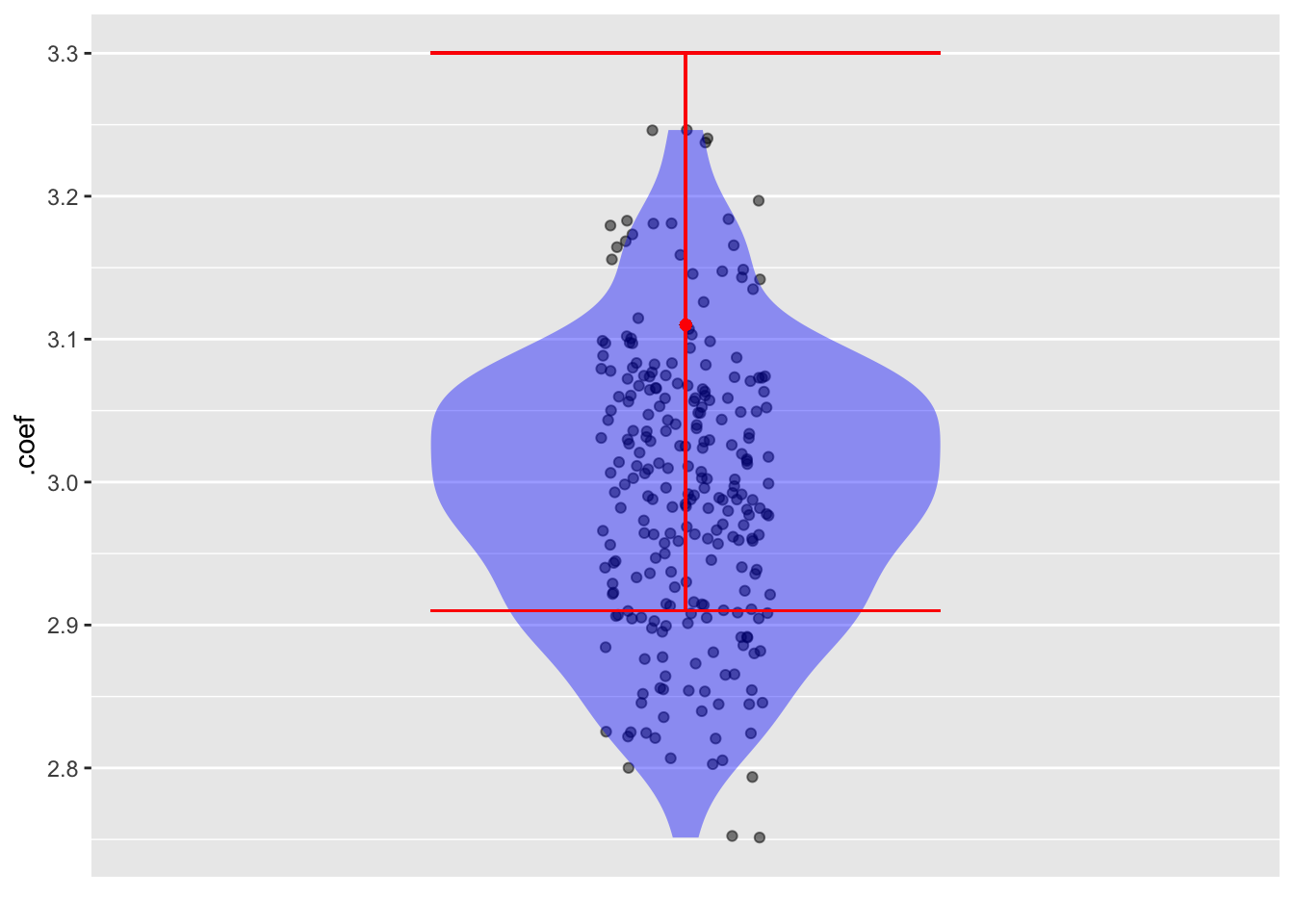
The confidence interval is centered on the coefficient from that sample. But that coefficient can come from anywhere in the simulated distribution. In this case, the original sample was from the upper end of the distribution.
Question: Although the location of the confidence interval from a sample is not necessarily centered close to the “true value” (which is 3.0 for sim_02), there is another aspect of the confidence interval that gives a good match to the distribution of trials of the simulation. What is that aspect?
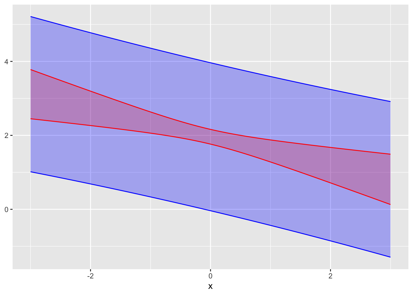
Exercise 28.3 The following graphs show confidence bands for the same model fitted to two samples of different sizes.

A. Do the two confidence bands (red and blue) plausibly come from the same model? Explain your reasoning. Answer: The two bands overlap substantially, so they are consistent with one another.
B. Which of the confidence bands comes from the larger sample, red or blue? Answer: Red. A larger sample produces smaller confidence intervals/bands.)
C. To judge from the graph, how large is the larger sample compared to the smaller one? Answer: The red band is about half as wide as the blue band. Since the width of the band goes as \(\sqrt{n}\), the sample for the red band is about four times as large as for the blue.
Exercise 28.4 In the graph, a confidence interval and a prediction interval from the same model are shown.
A. Which is the confidence interval, red or blue?
B. To judge from the graph, what is the standard deviation of the residuals from the model?
Exercise 28.5 The graph shows a confidence interval and a prediction interval.
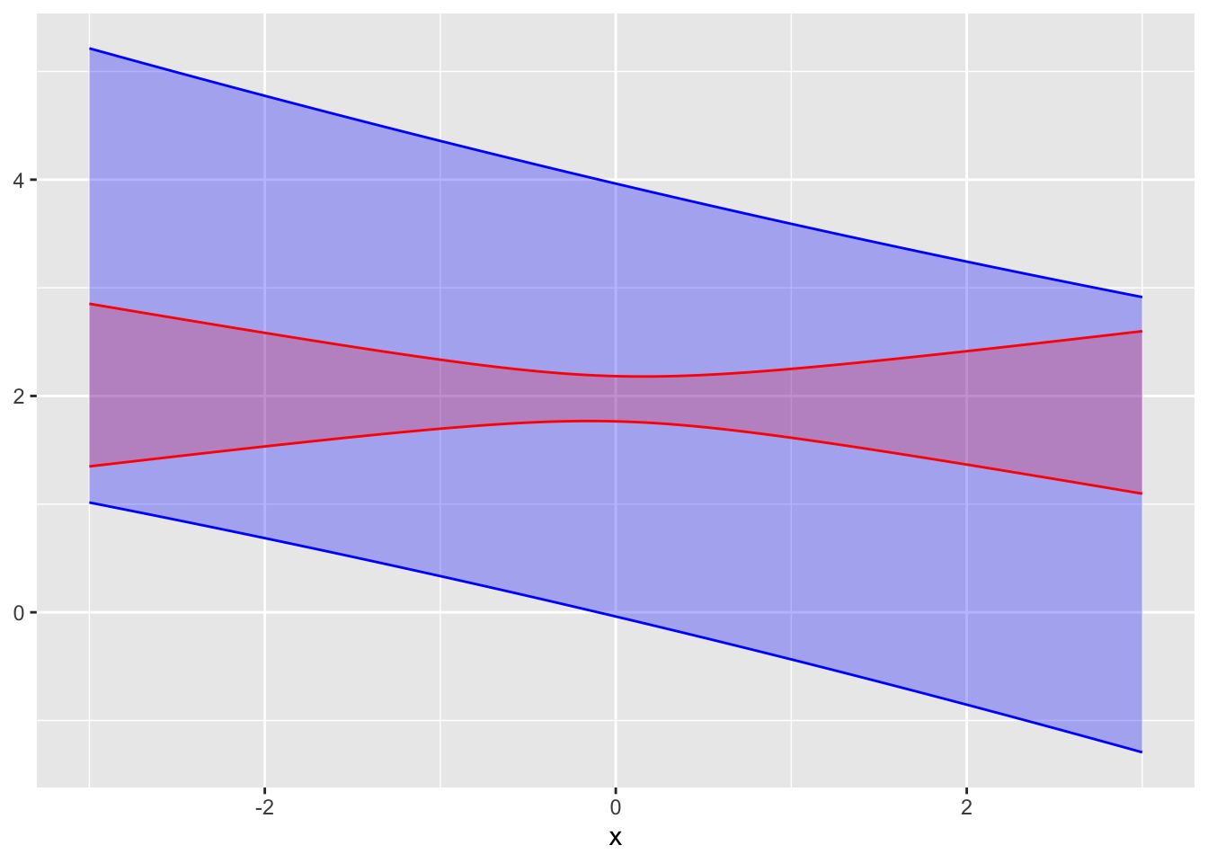
A. Which is the confidence interval, red or blue? Answer: Red. The confidence interval/band is always thinner than the prediction interval/band.
B. Do the confidence interval and the prediction come from the same sample of the same system? Explain your reasoning. Answer: No. If they came from the same system, the prediction band would be centered on the confidence band.
Exercise 28.6 An industrial process for making solar photovoltaics involves printing layers of doped silicon onto a large plastic substrate. The integrity of the final product varies from run to run. You are the manager of the production line and have asked the quality control technicians to measure the atmospheric humidity for each run to check if humidity is related to product integrity. Integrity must be at least 14 for the output of the product run to be accepted.
The graph shows the data from 50 production runs along with a prediction band from a model trained on the data.
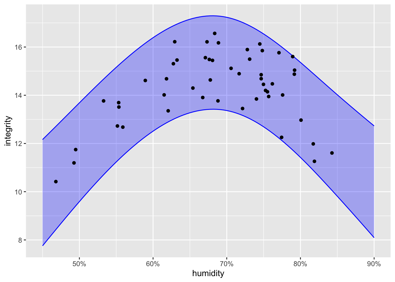
As manager, you have decided that the probability of the integrity being above 14 must be at least 75% in order to generate an appropriate production quantity without wasting too much material from the rejected production runs.
A. What is the interval of acceptable humidity levels in order to meet the above production standards?
B. As more production runs are made, more data will be collected. Based on what you know about prediction bands, will the top and bottom of the band become closer together as more data accumulates?
Short projects
Exercise 28.7 A 1995 article recounted an incident with a scallop fishing boat. In order to protect the fishery, the law requires that the average weight of scallops caught be larger than 1/36 pound. The particular ship involved returned to port with 11,000 bags of frozen scallops. The fisheries inspector randomly selected 18 bags as the ship was being unloaded, finding the average weight of the scallops in each of those bags. The resulting measurements are displayed below, in units of 1/36 pound. (That is, a value of 1 is exactly 1/36 pound while a value of 0.90 is \(\frac{0.90}{36}=0.025\) pound.)
Sample <- tibble::tribble(
  ~ scallops,
  0.93, 0.88, 0.85, 0.91, 0.91, 0.84, 0.90, 0.98, 0.88,
  0.89, 0.98, 0.87, 0.91, 0.92, 0.99, 1.14, 1.06, 0.93)
Sample |> model_train(scallops ~ 1) |> conf_interval(level=0.99)| term | .lwr | .coef | .upr |
|---|---|---|---|
| (Intercept) | 0.8802122 | 0.9316667 | 0.9831212 |
If the average of the 18 measurements is below 1.0, a penalty is imposed. For instance, an average of 0.97 leads to 40% confiscation of the cargo, while 0.93 and 0.89 incur to 95- and 100-percent confiscation respectively.
The inspection procedure—select 18 bags at random and calculate the mean weight of the scallops therein, penalize if that mean is below 1/36 pound—is an example of a “standard operating procedure.” The government inspector doesn’t need to know any statistics or make any judgment. Just count, weigh, and find the mean.
Designing the procedure presumably involves some collaboration between a fisheries expert (“What’s the minimum allowed weight per scallop? I need scallops to have a fighting chance of reaching reproductive age.”), a statistician (“How large should the sample size be to give the desired precision? If the precision is too poor, the penalty will be effectively arbitrary.”), and an inspector (“You want me to sample 200 bags? Not gonna happen.”)
A. Which of the numbers in the above report correspond to the mean weight per scallop (in units of 1/36 pound)?
There is a legal subtlety. If the regulations state, “Mean weight must be above 1/36 pound,” then those caught by the procedure have a legitimate claim to insist that there be a good statistical case that the evidence from the sample reliably relates to a violation.
B. Which of the numbers in the above report corresponds to a plausible upper limit on what the mean weight has been measured to be?
Back to the legal subtlety …. If the regulations state, “The mean weight per scallop from a random sample of 18 bags must be 1/36 pound or larger,” then the question of evidence doesn’t come up. After all, the goal isn’t necessarily that the mean be greater than 1/36th pound, but that the entire procedure be effective at regulating the fishery and fair to the fishermen. Suppose that the real goal is that scallops weigh, on average, more than 1/34 of a pound. In order to ensure that the sampling process doesn’t lead to unfair allegations, the nominal “1/36” minimum might reflect the need for some guard against false accusations.
C. Transpose the whole confidence interval to where it would be if the target were 1/34 of a pound (that is, \(\frac{1.06}{36}\). Does the confidence interval from a sample of 18 bags cross below 1.0?
An often-heard critique of such procedures is along the lines of, “How can a sample of 18 bags tell you anything about what’s going on in all 11,000 bags?” The answer is that the mean of 18 bags—on its own—doesn’t tell you how the result relates to the 11,000 bags. However, the mean with its confidence interval does convey what we know about the 11,000 bags from the sample of 18.
D. Suppose the procedure had been defined as sampling 100 bags, rather than 18. Using the numbers from the above report, estimate in \(\pm\) format how wide the confidence interval would be.
Exercise 28.8 If you have ever hiked near the crest of a mountain, you may have noticed that the vegetation can be substantially different from one side of the crest to another. To study this question, we will look at the Calif_precip data frame, which records the amount of precipitation at 30 stations scattered across the state, recording precipitation, altitude, latitude, and orientation of the slope as “W” or “L”. (We will also get rid of two outlier stations.)
modW <-
  Calif_precip |>
  filter(orientation=="W", station != "Cresent City") |>
  model_train(precip ~  altitude + latitude)

modL <- Calif_precip |>
  filter(orientation=="L", station != "Tule Lake") |>
model_train(precip ~ altitude + latitude) 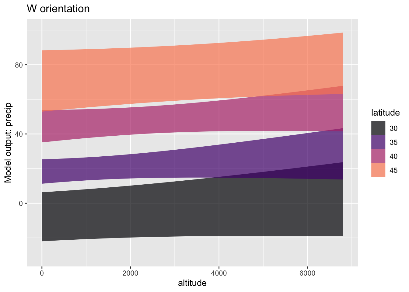
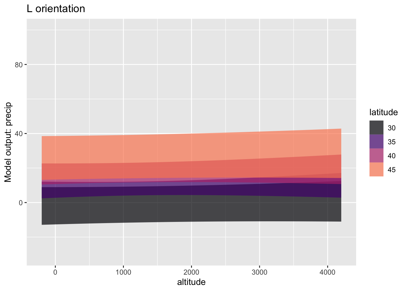
A. You can see that the W model and the L model are very different. One difference is that the precipitation is much higher for the W stations than the L stations. How does the higher precipitation for W show up in the graphs? (Hint: Don’t overthink the question!)
B. Another difference between the models has to do with the confidence bands. The bands for the L stations are pretty much flat while those for the W stations tend to slope upwards.
i. What about the altitude confidence intervals on `modW` and `modL` corresponds to the difference?
ii. Calculate R^2^ for both the L model and the W model. What do the different values of R^2^ suggest about how much of the explanation of `precip` is accounted for by each model?Exercise 28.9
MAKE THIS ABOUT WHAT THE SAMPLE SIZE NEEDS TO BE to see the difference in walking times.
This demonstration is motivated by an experience during one of my early-morning walks. Due to recent seasonal flooding, a 100-yard segment of the quiet, riverside road I often take was covered with sand. The concrete curbs remained in place so I stepped up to the curb to keep up my usual pace. I wondered how close to my regular pace I could walk on the curb, which was plenty wide: about 10 inches.
Imagine studying the matter more generally, assembling a group of people and measuring how much time it takes to walk 100 yards, either on the road surface or the relatively narrow curve. Suppose the ostensible purpose of the experiment is to develop a “handicap,” as in golf, for curve walking. But my reason for including the matter in a statistics text is to demonstrate statistical thinking.
In the spirit of demonstration, we will simulate the situation. Each simulated person will complete the 100-yard walk twice, once on the road surface and once on the curb. The people differ one from the other. We will use \(70 \pm 15\) seconds road-walking time and slow down the pace by 15% (\(\pm 6\)%) on average when curb walking. There will also be a random factor affecting each walk, say \(\pm 2\) seconds.
walking_sim <- datasim_make(
  person_id <- paste0("ID-", round(runif(n, 10000,100000))),
  .road <- 70 + rnorm(n, sd=15/2),
  .curb <- .road*(1 + 0.15 + rnorm(n, sd=0.03)),
  road <- .road*(1 + rnorm(n, sd=.02/2)),
  curb <- .curb*(1 + rnorm(n, sd=(.02/2)))
)
LET’S Look at the confidence interval for two models
Walks <- walking_sim |> datasim_run(n=10) |>
  tidyr::pivot_longer(-person_id,
                      names_to = "condition",
                      values_to = "time")
Walks |> model_train(time ~ condition) |>
conf_interval()| term | .lwr | .coef | .upr |
|---|---|---|---|
| (Intercept) | 73.7 | 80.0 | 86.200 |
| conditionroad | -18.7 | -9.8 | -0.941 |
Walks |> model_train(time ~ condition + person_id) |>
conf_interval()| term | .lwr | .coef | .upr |
|---|---|---|---|
| (Intercept) | 70.800 | 74.30 | 77.90 |
| conditionroad | -11.900 | -9.80 | -7.66 |
| person_idID-30353 | -2.210 | 2.59 | 7.39 |
| person_idID-31011 | -2.900 | 1.90 | 6.70 |
| person_idID-34917 | -16.800 | -12.00 | -7.16 |
| person_idID-52467 | 8.380 | 13.20 | 18.00 |
| person_idID-60634 | 1.510 | 6.31 | 11.10 |
| person_idID-64511 | -2.580 | 2.21 | 7.01 |
| person_idID-79516 | 12.700 | 17.50 | 22.30 |
| person_idID-89160 | -0.202 | 4.60 | 9.39 |
| person_idID-98520 | 15.100 | 19.90 | 24.70 |
Enrichment topics
Enrichment topic 28.1: Where do priors come from?
The use of Bayes’ Rule (formula 28.3) to transform a prior into a posterior based on the likelihood of observed data is a mathematically correct application of probability. It is used extensively in engineering, machine learning and artificial intelligence, and statistics, among other fields. Some neuroscientists argue that neurons provide a biological implementation of an approximation to Bayes’ Rule.
The Theory That Would Not Die: How Bayes’ Rule Cracked the Enigma Code, Hunted Down Russian Submarines, and Emerged Triumphant from Two Centuries of Controversy, by Sharon Bertsch McGrayne, provides a readable history. As the last words in the book’s title indicate, despite being mathematically correct, Bayes’ Rule has been a focus of disagreement among statisticians. The disagreement created a schism in statistical thought. The Bayesians are on one side, the other side comprises the Frequentists.
The name “frequentist” comes from a sensible-sounding definition of probability as rooted in long-run counts (“frequencies”) of the outcomes of random trials. A trivial example: the frequentist account of a coin flip is that the probability of heads is 1/2 because, if you were to flip a coin many, many times, you would find that heads come up about as often as tails. According to frequentists, a hypothesis is either true or false; there is no meaningful sense of the probability of a hypothesis because there is only one reality; you can’t sample from competing realities.
The frequentists dominated the development of statistical theory through the 1950s. Most of the techniques covered in conventional statistics courses stem from frequentist theorizing. One of the most famous frequentist techniques is hypothesis testing, the subject of Lesson 29.
Today, mainstream statisticians see the schism between Frequentists and Bayesians as an unfortunate chapter in statististical history and view hypothesis testing as a dubious way to engage scientific questions (albeit one that still has power, controversially, as a gateway to research publication).
Frequentists note that beliefs differ from one person to the next and that priors may have little or no evidence behind them. Bayesians acknowledge that beliefs differ, but point out that a person disagreeing with a conclusion based on a questionable prior can themselves propose an alternative prior and find the posterior that corresponds to this alternative. Indeed, as illustrated in Enrichment topic 28.3, one can offer a range of priors and let the accumulating evidence create a narrower set of posteriors.
Or, prior probability for a sports team that was no good last year, but has had an excellent first three games.
DRAFT: Disease prevalence, general accident rate, long-term weather or sports statistics.
Enrichment topic 28.2: Accumulating evidence (in Draft)
THE CYCLE OF ACCUMULATION. Let’s look at biopsy that follows a mammogram, both with a \(\Ptest\) and a \(\Ntest\) result.
Enrichment topic 28.3: Multiple hypotheses (in Draft).
The previous section showed the transformation from prior to posterior when there are only two hypotheses. But Bayesian thinking applies to situations with any number of hypotheses.
Suppose we have \(N\) hypotheses, which we will denote \({\cal H}_1, {\cal H}_2, \ldots, {\cal H}_N\).
Since there are multiple hypotheses, it’s not clear how odds will apply. So instead of stating priors and posteriors as odds, we will write them as relative probabilities. We’ll write the prior for each hypothesis as \(prior({\cal H}_i)\) and the posterior as \(posterior({\cal H}_i)\).
Now an observation is made. Let’s call it \(\mathbb{X}\). This observation will drive the transformation of our priors into our posteriors. As before, the transformation involves the likelihood of \(\mathbb{X}\) under the relative hypotheses. That is, \({\cal L}_{\cal H_i}(\mathbb{X})\). The calculation is simply
\[posterior({\cal H_i}) = {\cal L}_{\cal H_i}(\mathbb{X}) \times\ prior({\cal H_i}) \ \text{in relative probability form}\]
If you want to convert the posterior from a relative probability into an ordinary probability (between 0 and 1), you need to collect up the posteriors for all of the hypotheses. The notation \(p(\cal H_i\given \mathbb X)\) is conventional, where the posterior nature of the probability is indicated by the \(\given \mathbb X)\). Here’s the formula:
\[p(\cal H_i\given \mathbb X) = \frac{posterior(\cal H_i)}{posterior(\cal H_1) + posterior(\cal H_2) + \cdots + posterior(\cal H_N)}\]
Example: Car safety Maybe move the example using the exponential distribution from the Likelihood Lesson to here.
Note: There are specialized methods of Bayesian statistics and whole courses on the topic. An excellent online course is Statistical Rethinking.
Enrichment topic 28.4: Prior for schizophrenia?
Being a statistician, I am often approached by friends or acquaintances who have recently gotten a “positive” result on a medical screening test, for example cholesterol testing or prostate-specific antigen (PSA). They want to know how likely it is that they have the condition—heart disease or prostate cancer—being screened for. Before I can answer, I have to ask them an important question: How did you come to have the test? I want to know if the test was done as part of a general screening or if the test was done because of some relevant symptoms.
To illustrate why the matters of symptoms is important, consider a real-world test for schizophrenia.
In 1981, President Reagan was among four people shot by John Hinkley, Jr. as they were leaving a speaking engagement at a D.C. hotel. At trial, Hinckley’s lawyer presented an “insanity” defense, there being a longstanding legal principle that only people in control of their actions can be convicted of a crime.
As part of the evidence, Hinkley’s defense team sought to present a CAT scan showing atrophy in Hinkley’s brain. About 30% of schizophrenics had such atrophy, compared to only 2% of the non-schizophrenic population. Both of these are likelihoods, that is, a probability of what’s observed given the state of the subject.
A. Based on the above, do you think the CAT scan would be strong evidence of schizophrenia?
A proper calculation of the probability that a person with atrophy is schizophrenic depends on the prevalence of schizophrenia. This was estimated at about 1.5% of the US population.
Calculating the probability of the subject’s state given the observation of atrophy involves comparing two quantities, both of which have the form of a likelihood times a prevalence.
- Evidence in favor of schizophrenia: \[\underbrace{30\%}_\text{likelihood} \times \underbrace{1.5\%}_\text{prevalence} = 0.45\%\]
- Evidence against schizophrenia: \[\underbrace{2\%}_\text{likelihood} \times \underbrace{98.5\%}_\text{prevalence} = 1.97\%\] The probability of schizophrenia given atrophy compares the evidence for schizophrenia to the total amount of evidence: \[\frac{0.45\%}{1.97\% + 0.45\%} = 18.6\%\ .\] Based just on the result of the test for atrophy, Hinkley was not very likely to be a schizophrenic.
This is where the “How did you come to have the test?” question comes in.
For a person without symptoms, the 18.6% calculation is on target. But Hinkley had very definite symptoms: he had attempted an assassination. (Also, Hinkley’s motivation for the attempt was to impress actress Jody Foster, to “win your heart and live out the rest of my life with you.)
The prevalence of of schizophrenia among prisoners convicted of fatal violence is estimated at about 10 times that of the general population. Presumably, it is even higher among those prisoners who have other symptoms of schizophrenia.
B. Repeat the “evidence for” and “against” schizophrenia, but updated for a prevalence of 20% instead of the original 1.5%. Has this substantially change the calculated probability of schizophrenia?
Epilogue: Hinkley was found not guilty by virtue of insanity. He was given convalescent leave from the mental hospital in 2016 and released entirely in 2022.
Note: This question is based on a discussion in the July 1984 “Misapplications Reviews” column of INTERFACES **14(4):48-52.
Enrichment topic 28.5: Screening tests
One important use for tests such as the one we described is “medical screening.” Screening is applied to members of the general population who display no relevant symptoms and have no particular reason to believe they might be \(\Sick\). Familiar examples of tests used for screening: mammography for breast cancer, PSA for prostate cancer, Pap smears for cervical cancer. Screening also occurs in non-medical settings, for instance drug tests or criminal background checks required by employees for current or prospective workers.
The difference between screening settings and non-screening settings is a matter of degree. The number used to quantify the setting is called the “prevalence,” which is the fraction of people in the test-taking group who are \(\Sick\).
- Accumulating evidence. THE CYCLE OF ACCUMULATION. Let’s look at biopsy that follows a mammogram, both with a \(\Ptest\) and a \(\Ntest\) result.