Chapter 7 Data Wrangling
When data are in glyph-ready form it is straightforward to construct data graphics using the concepts and techniques in Chapters 5 and 6. First, you choose an appropriate sort of glyph: dots, stars, bars, countries, etc. Next, select which variables are to be mapped to the various aesthetics for that glyph. Then let the computer do the drawing.
On occasion, data will arrive in glyph-ready form. More typically, you have to wrangle the data into the glyph-ready form appropriate for your own purpose.
Example: Counting the ballots
Table 7.1 records the choice of each of 80101 individual voters in the 2013 mayoral election in Minneapolis, MN, USA.
Table 7.1: The choices of each voter in the mayoral election. See Minneapolis2013 in the dcData package.
| Precinct | First | Ward |
|---|---|---|
| P-10 | BETSY HODGES | W-7 |
| P-06 | BOB FINE | W-10 |
| P-09 | KURTIS W. HANNA | W-10 |
| P-05 | BETSY HODGES | W-13 |
| P-01 | DON SAMUELS | W-5 |
| P-04 | undervote | W-6 |
| … and so on for 80,101 rows altogether. |
The primary use for data like Table 7.1 is to determine how many votes were given to each candidate. Counting the votes for each candidate is a simple wrangling task that transforms the ballot data (Table 7.1) into a glyph-ready form (Table 7.2 right) that makes the answer obvious. The count information is still latent in the raw ballot data; it is not yet in a form where it is easily seen.
Table 7.2: The number of votes for each candidate. This has been wrangled from Table 7.1 into a glyph-ready form, that is, a form in which the information sought after is readily seen.
| candidate | count |
|---|---|
| BETSY HODGES | 28935 |
| MARK ANDREW | 19584 |
| DON SAMUELS | 8335 |
| CAM WINTON | 7511 |
| JACKIE CHERRYHOMES | 3524 |
| BOB FINE | 2094 |
| … and so on for 38 rows altogether. |
The instructions for carrying out the wrangling are simple to give in English: Count the number of ballots that each candidate received and sort from highest to lowest. To carry out the process on a computer, you need to express this idea in a form the computer can carry out.
7.1 Planning your wrangling
Before you start wrangling data, it’s crucial to envision what the goal is to be. In general, the purpose of wrangling is to take the data you have at hand and put it into glyph-ready form. But glyph-ready for what? This is something you, the data analyst, need to determine based on your own objectives.
Example: Demographic patterns of smoking
Table 7.3 has variables indicating each person’s age, sex, and whether he or she smokes.
Table 7.3: The NCHS data from the dcData package. In NCHS, the case is an individual person.
| age | sex | smoker |
|---|---|---|
| 2 | female | no |
| 77 | male | no |
| 10 | female | no |
| 1 | male | no |
| 49 | male | yes |
| 19 | female | no |
| … and so on for 29,375 rows altogether. |
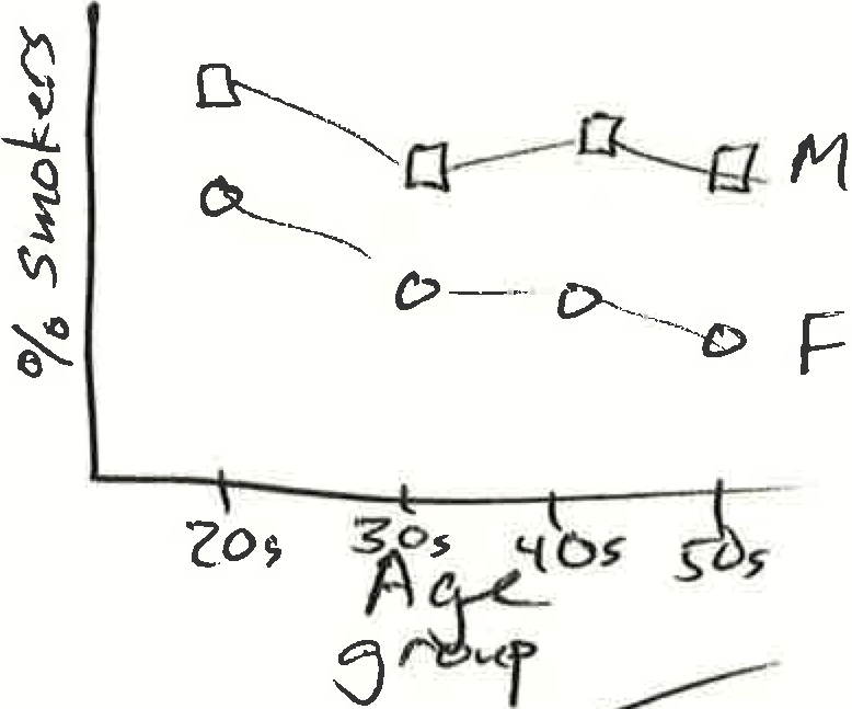
Suppose you want to use NCHS to explore the links between smoking and age. Often you will have some kind of presentation graphic in mind. Making an informal sketch like Figure 7.1 can be a helpful way to chart a path for data wrangling. The sketch can be based on your imagination of what the data might show. Even so, the sketch contains important information. For instance, from the sketch you can determine what a single glyph represents. As always, each glyph will be one case in the glyph-ready data. In this sketch, the glyph describes a group of people — people of one sex in one age group. This differs from the cases in NCHS: individual people.
Figure 7.1: A made-up depiction of trends in the fraction of people of different ages who smoke.
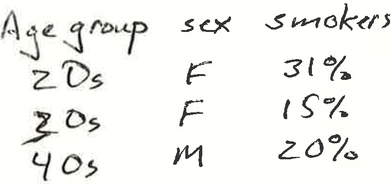
To make your goal for data wrangling even more explicit, rough out the form of the glyph-ready data frame, as in Figure 7.2. Don’t worry about calculating precise data values; the computer will do that after you have implemented your data wrangling plan.
Figure 7.2: A sketch of the form of glyph-ready data corresponding to Figure 7.1. For each aesthetic in Figure 7.1 there is one variable in the glyph-ready table.
The glyph-ready data for that graph will has a form like the rough table in Figure 7.2. That glyph-ready form is your target.
Once you have a target glyph-ready format in mind, use plain English to plan the individual data wrangling steps. For instance, a plan for wrangling Table 7.3 into Table 7.2 might look like this:
- Turn the age in years into a new variable, the age group (in decades).
- Drop the people under 20-years old.
- Divide up the table into separate groups for each age decade and sex.
- For each of those groups, count the number of people and the number of people who smoke. Divide one by the other to get the fraction who smoke.
Each of these step would be easy enough to do by hand (if you had the time and patience to work through 31126 cases in NCHS). To get the computer to do the work for you, you have to be able to describe each process to the computer. The next sections present a framework for describing wrangling operations that can work for both the human describing the wrangling and the computer that will carry out the calculations.
7.2 A Framework for Data Wrangling
Over the last half century, researchers have identified a small set of patterns that can be used to describe a wrangling process. Because this set is small, it’s feasible for you to learn quickly what you need to describe the wrangling you have planned.
As you know, doing something in R is accomplished using functions. A function takes one or more inputs (the “arguments”) and returns an output. In thinking about data wrangling, it helps to consider these potential forms for inputs and outputs:
- A data frame, a collection of variables and cases.
- A variable, just a single one from the collection in a data frame.
- A scalar, a single number or character string.
There are three broad families of functions involved in data wrangling. The families differ in what form of input they take in and what form they return.
- Reduction functions take a variable as input and return a scalar.
- Transformation functions take one or more existing variables as input and return a new variable.
- Data verbs take an existing data frame as input and return a new data frame.
Each step in data wrangling involves a data verb and one or more reduction or transformation functions.
7.3 Reduction Functions
Reduction functions summarize or reduce a variable to scalar form. You are likely familiar with several reduction functions:
mean()— find a single typical valuesum()— add up numbers into a totaln()— find how many cases there are
Some other frequently used reduction functions:
min()andmax()— find the smallest and largest value in a variablemedian(),sd()and other functions used in statisticsn_distinct()— how many different levels are there among the cases
7.4 Transformation Functions
Transformation functions take one or more variables as input and return a new variable. In contrast to reduction functions, which produce a single number — a scalar — by combining all the cases, transformation functions produce a result for each individual case.
Often, transformations are mathematical operations, for instance:
weight / heightlog10( population )round( age )
Other transformation functions include numerical and character comparisons, as in Table 7.4.
Table 7.4: Some of the functions used to compare values.
| Function | Meaning | Example |
|---|---|---|
| For numerical comparisons | ||
<
|
less than |
age
|
>
|
greater than |
age
|
==
|
matches exactly |
age == 39
|
%in%
|
is one of |
age %in% c(18, 19, 20)
|
| For character strings | ||
<
|
alphabetically before |
name
|
>
|
alphabetically after |
name
|
==
|
matches exactly |
name == "Jon"
|
%in%
|
is one of |
name %in% c("Abby", "Abe")
|
Another important operation, ifelse() allows you to translate each value in a variable to one of two values, depending on the result of a comparison. For instance
ifelse(age >= 18, "voter", "non-voter")
7.5 Data Verbs
Data verbs carry out an operation on a data frame and return a new data frame. Some data verbs involve the modification of variables, the creation of new variables, or the deletion of existing ones. Other data verbs involve changing the meaning of a case or adding or deleting cases.
In addition to a data frame input, each data verb takes additional arguments that provide the specifics of the operation. Very often, these specifics involve reduction and transformation functions.
There are about a dozen data verbs that are commonly used. Additional data verbs will be introduced in Chapter 10 and beyond, but lots of interesting questions can be investigated with just these two:
summarise()— turns multiple cases into a single case using reduction functions. “Aggregate” is synonym for “summarise.”group_by()— modifies the action of reduction functions so that they give a single value for different groups of cases in a data frame.
To illustrate the uses of summarise(), look at the WorldCities data frame (in the dcData package) with information about the most populous cities in each country. Table 7.5 is a subset of the variables:
Table 7.5: World cities
| name | population | country | latitude | longitude |
|---|---|---|---|---|
| Shanghai | 14608512 | CN | 31.22222 | 121.45806 |
| Buenos Aires | 13076300 | AR | -34.61315 | -58.37723 |
| Mumbai | 12691836 | IN | 19.07283 | 72.88261 |
| Mexico City | 12294193 | MX | 19.42847 | -99.12766 |
| Karachi | 11624219 | PK | 24.90560 | 67.08220 |
| Istanbul | 11174257 | TR | 41.01384 | 28.94966 |
| Delhi | 10927986 | IN | 28.65381 | 77.22897 |
| Manila | 10444527 | PH | 14.60420 | 120.98220 |
| Moscow | 10381222 | RU | 55.75222 | 37.61556 |
| Dhaka | 10356500 | BD | 23.71040 | 90.40744 |
| … and so on for 23,018 rows altogether. |
A simple summary of the data is a count of the number of cities.
| count |
|---|
| 23018 |
The reduction function is n(). The expression count = n() means that the output data frame should have a variable named count containing the results of n(). The n() function doesn’t take any arguments.
Perhaps you want to know the total population in these cities, or the average population per city or the smallest city in the table, as in Table 7.6.
WorldCities %>%
  summarise(averPop  = mean(population, na.rm=TRUE),
            totalPop = sum(population, na.rm=TRUE),
            smallest = min(population, na.rm=TRUE))
Table 7.6: Summary statistics of the population of world cities
| averPop | totalPop | smallest |
|---|---|---|
| 112624.8 | 2592396767 | 0 |
The average city on the list has about 110,000 people. The total population of people living in these cities is about 2.6 billion — a bit more than one-third of the world population. The smallest city has … zero people! Evidently, the WorldCities data frame has one or more cases that are not really cities.
Some things to notice about the use of summarise():
- The chaining syntax,
%>%has been used to pass the first argument tosummarize(). This will be useful later on, when there is more than one step in a transfiguration. It’s OK to end a line with%>%, but never start a line with it. - The output of
summarise()is a data frame. (In this example the output has only one case, but it is still a data frame.) summarise()takes named arguments. The name of an argument is taken as the name of the corresponding variable created bysummarise().
7.6 group_by
The group_by() data verb sets things up so that other data verbs will perform their action on a group-by-group basis. For instance, Table 7.7 shows the number of cities in WorldCities broken down by country.
Table 7.7: The number of cities in each country listed in WorldCities.
| country | count |
|---|---|
| AD | 2 |
| AE | 12 |
| AF | 50 |
| AG | 1 |
| AI | 1 |
| AL | 20 |
| … and so on for 243 rows altogether. |
The group_by() verb should always be followed by another verb — summarise() in the above example. group_by() is the way to indicate to the following verbs that reduction operations should be performed on a group-wise basis.
Using group_by() along with summarise() and n(), provides a basis for counting up the number of cases in groups and subgroups, or for calculating group-wise statistics.
Note that the functions used within arguments to summarise() — functions such as n(), max(), sum(), etc. — are not data verbs. A data verb takes a data frame as input and returns a transfigured data frame as output. In contrast, the reduction functions, n(), sum(), and so on, take a variable as input and return a single number as output.
7.7 Is That All?
The summarise() and group_by() data verbs are team players; they work best in combination with other data verbs. Once you learn those data verbs, particularly filter() and mutate(), you’ll be able to carry out many more operations. The richness of the data-verb system comes from the ways the different verbs can be combined together.
Example: Counting Births
Suppose you want to create a graph like Figure 7.3 to examine the relative number of male and female births over time.
Figure 7.3: Births registered by the US Social Security Administration over the years.
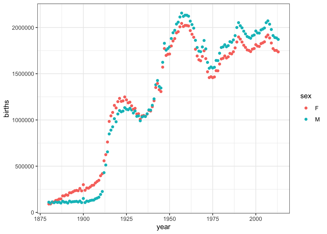
The BabyNames data frame contains this information implicitly. Before the information can be graphed, you need to wrangle the existing data frame into glyph-ready form.
Table 7.11: The BabyNames data frame
| name | sex | count | year |
|---|---|---|---|
| Juana | F | 121 | 1956 |
| Stamatia | F | 5 | 1981 |
| Kenesha | F | 16 | 2004 |
| Aubreigh | F | 63 | 2010 |
| Yadriel | M | 17 | 2012 |
| Mariam | F | 52 | 1922 |
| … and so on for 1,792,091 rows altogether. |
The particular wrangling needed here is to calculate the sum of count for each sex in each year. Here’s one way to do this.
Table 7.12: The data frame YearlyBirths comes from BabyNames wrangled into counts of births each year.
| year | sex | births |
|---|---|---|
| 1880 | F | 90993 |
| 1880 | M | 110491 |
| 1881 | F | 91954 |
| 1881 | M | 100746 |
| 1882 | F | 107850 |
| 1882 | M | 113687 |
| … and so on for 268 rows altogether. |
YearlyBirths is in glyph-ready form. Using YearlyBirths, drawing Figure 7.3 is a matter of assigning variables to graphical aesthetics: year to the \(x\)-axis, births to the \(y\)-axis, and sex to dot color.
7.8 Exercises
Problem 7.1: For each of the operations listed here, say whether it involves a transformation function or a reduction function or neither.
- Determine the 3rd largest.
- Determine the 3rd and 4th largest values.
- Determine the number of cases.
- Determine whether a year is a leap year.
- Determine whether a date is a legal holiday.
- Determine the range of a set, that is, the max minus the min.
- Determine which day of the week (e.g., Sun, Mon, …) a given date is.
- Find the time interval in days spanned by a set of dates.
Problem 7.2: Each of these statements have an error. It might be an error in syntax or an error in the way the data tables are used, etc. Describe what each expression apparently attempts to do, as well as the error(s) that cause them to fail.
BabyNames %>%
  group_by( "First" ) %>%
  summarise( votesReceived=n() )
Tmp <- group_by(BabyNames, year, sex ) %>%
summarise( Tmp, totalBirths=sum(count))Tmp <- group_by(BabyNames, year, sex)
summarise( BabyNames, totalBirths=sum(count) )Problem 7.3: Using the Minneapolis2013 data table in the dcData package, answer these questions:
- How many cases are there?
- Who were the top 5 candidates in the
Secondvote selections. - How many ballots are marked “undervote” in
Firstchoice selections?Secondchoice selections?Thirdchoice selections?
- What are the top 3 combinations of
FirstandSecondvote selections? (That is, of all the possible ways a voter might have marked his or her first and second choices, which received the highest number of votes?) - Which
Precincthad the highest number of ballots cast?
Problem 7.4: Each of these statements has an error. It might be an error in syntax or an error in the way the data tables are used, etc. Write down a correct version of the statement.
BabyNames %>%
  group_by(BabyNames, year, sex) %>%
  summarise(BabyNames, total = sum(count))
ZipGeography <-
group_by(State) %>%
summarise(pop = sum(Population))Minneapolis2013 %>%
group_by(First) ->
summarise(voteReceived = n())summarise(votesReceived = n()) %<%
group_by(First) <- Minneapolis2013Problem 7.5: The data verbs group_by() and summarise() are very frequently used in combination. Experiment with the R code, help documentation, etc to investigate each of the following.
- How has the result
VoterData_Aapparently been modified when compared to the originalMinneapolis2013data? What does a case represent inVoterData_A?
VoterData_A <-
  Minneapolis2013 %>%
group_by(First, Second)- How has the result
VoterData_Bapparently been modified when compared to the originalMinneapolis2013data? What does a case represent inVoterData_B?
VoterData_B <-
  Minneapolis2013 %>%
summarise( total = n() )- How has the result
VoterData_Capparently been modified when compared to the originalMinneapolis2013data? What does a case represent inVoterData_C?
VoterData_C <-
  Minneapolis2013 %>%
  group_by(First, Second) %>%
summarise( total = n() )- Here, the
group_by()andsummarise()steps are reversed and now the result is an error indicating that “ColumnFirstis unknown.” Clearly the variableFirstexisted in theMinneapolis2013data frame, why is it now unknown?
## Error: Must group by variables found in `.data`.
## * Column `First` is not found.
## * Column `Second` is not found.
Problem 7.6: Using the ZipGeography data
Find the total land area and population in each state.
Make a scatter plot showing the relationship between land area and population for each state.
Make a choropleth map showing the population of each state.
Make a choropleth map showing the population per unit area of each state.
Problem 7.7: Imagine a data table, Patients, with categorical variables name, diagnosis, sex, and quantitative variable age.
You have a statement in the form
Patients %>%
  group_by(  **SOME_VARIABLES** ) %>%
  summarise(count = n(), meanAge = mean(age))
Replacing **SOME_VARIABLES** with each of the following, tell what variables will appear in the output
sexdiagnosissex,diagnosisage,diagnosisage
Problem 7.8: Use the ZipDemography data from the dcData package for the following tasks.
- Make a scatter plot showing the relationship, if any, between the number of
Foreignbornpeople in a zip code and the number whoSpeakalanguageotherthanEnglishathome5yearsandover. (Please note that such long variable names ought to be avoided as a matter of good style.)
Warning: do NOT attempt to facet by ZIP code as you explore solutions. Doing so is very computationally intense (i.e., takes a long time if it finishes at all) only to show that one facet for each ZIP code is not a useful data visualization.
- Explain what would keep you, at this point, from calculating the fraction of people in each state who have a
Bachelorsdegreeorhigher. Say how you would go about constructing such a plot — but don’t actually do it! Too much work.