Chapter 16 Data Scraping and Intake Methods
“Every easy data format is alike. Every difficult data format is difficult in its own way.” — inspired by Leo Tolstoy
The wrangling and visualization techniques in this book are designed for working with data in a tidy data frame format. Often, the data you encounter are in some other format. An early step in working with such formats is to translate them into one or more data frames. This process is called data scraping. Data scraping: Gathering data from sources that are not already in data frame format. It usually refers to translating from formats used by web browsers to data table form. Here it’s used in a more general sense.
Likewise, data often have errors that stem from blunders in data entry or from deficiencies in the way data is stored or coded. Correcting such errors is called data cleaning. Correcting errors or deficiencies in the way data is stored or coded.
16.1 Data Frame Friendly Formats
Many formats for data are essentially equivalent to data frames. When you come across data in a format that you don’t recognize, it’s worth checking whether it’s one of the data frame friendly formats. Sometimes the filename extension provides an indication. Here are several, each with a brief description:
- CSV file. A non-proprietary text format that is widely used for data exchange between different software packages.
- data sources in a technical software-package specific format:
- Octave (and through that, MATLAB) widely used in engineering and physics.
- Stata, commonly used for economic research
- SPSS, commonly used for social science research
- Minitab, often used in business practices
- SAS, often used for mid-sized or large data sets
- Epi, used by the Centers for Disease Control (CDC) for health and epidemiology data.
- Relational databases. This is the form that much of institutional, actively updated data are stored in. This includes business transaction records, government records, and so on.
- Excel, a set of proprietary spreadsheet formats heavily used in business. Watch out, though. Just because something is stored in an Excel format doesn’t mean it’s a data frame. Excel is sometimes used as a kind of table cloth for writing down data with no particular scheme in mind.
- Web-related
- HTML
<table>format - JSON
- XML
- Google spreadsheets published as HTML
- Application Programming Interfaces (APIs); e.g., Socratic Open Data API (SODA)
- HTML
The particular software and techniques for reading data in one of these formats, varies depending on the format. For Excel or Google spreadsheet data, it’s often sufficient to use the application software to export the data as a CSV file. There are also R packages for reading directly from an Excel spreadsheet, which is useful if the spreadsheet is being updated frequently.
For the technical software package formats, the foreign R package provides useful reading and writing functions. For relational databases, even if they are on a remote server, there are several useful R packages, including dplyr and data.table.
CSV and HTML <table> formats are frequently encountered. The next subsections give a bit more detail about how to read them into the R environment.
16.2 CSV
CSV stands for comma-separated values. It’s a text format that can be read with a huge variety of software. It has a data frame format, with the values of variables in each case separated by commas. Here’s an example of the first several lines of a CSV file:
"name","sex","count","year"
"Mary","F",7065,1880
"Anna","F",2604,1880
"Emma","F",2003,1880
"Elizabeth","F",1939,1880
The top row usually (but not always) contains the variable names. Quotation marks are often used at the start and end of character strings; these quotation marks are not part of the content of the string. CSV files are often named with the .csv suffix, it’s also common for them to be named with .txt or other things. You will also see characters other than commas being used to delimit the fields: tabs, vertical bars, and semicolons are particularly common.
Since reading CSV spreadsheet data is so common, many package authors have provided functions for this task. read.csv() in the base package is perhaps the most widely used, but not the best.
Table 16.1: Several functions for reading .csv files. To the user, they differ in flexibility in responding to the details of data file formats, whether they read Internet files directly, and speed.
| Function | Package | Adapts to delimiter | Accepts Web URL | Fast |
|---|---|---|---|---|
read.csv()
|
base
|
No | No | No |
read_csv()
|
readr
|
No | Yes | Yes |
fread()
|
data.table
|
Yes | Yes | Yes |
read.file
|
mosaic
|
Yes | Yes | Yes |
readr::read_csv() is the function primarily adopted in this book for reading CSV files, although data.table::fread() and mosaic::read.file() are useful alternatives. In contrast to base::read.csv(), all three of these work for both files on your computer and those available on the Internet via a URL. For instance, here’s a way to access a .csv file over the Internet.
# Remember the quotes around the URL character string.
webURL <- "https://mdbeckman.github.io/dcSupplement/data/houses-for-sale.csv"
MyDataTable <- read_csv(webURL)

MyDataTable %>%
  select(price, bedrooms,
         bathrooms, fuel, air_cond, construction)
Table 16.2: The data set at https://mdbeckman.github.io/dcSupplement/data/houses-for-sale.csv
| price | bedrooms | bathrooms | fuel | air_cond | construction |
|---|---|---|---|---|---|
| 132500 | 2 | 1.0 | 3 | 0 | 0 |
| 181115 | 3 | 2.5 | 2 | 0 | 0 |
| 109000 | 4 | 1.0 | 2 | 0 | 0 |
| 155000 | 3 | 1.5 | 2 | 0 | 0 |
| 86060 | 2 | 1.0 | 2 | 1 | 1 |
| 120000 | 4 | 1.0 | 2 | 0 | 0 |
| … and so on for 1,728 rows altogether. |
Just as reading a data file from the Internet uses a URL, reading a file on your computer uses a complete name, including the path to the file. Most people are used to using a mouse-based selector to access their files. The file.choose() function enables you to select a file in the familiar way, returning a character string with the file and path name. You can then call an appropriate function to read the file identified by that character string. To illustrate:
file_name <- file.choose() # then navigate and click on your file

MyDataTable2 <-
  data.table::fread(file_name)
Useful arguments to data.table::fread():
nrows = 0— just read the variable names. This is helpful when you are checking into the format and variable names of a data source. Of course, you might also want to look at a few rows of data, by settingnrowsto a small positive integer, e.g.nrows = 5.select = c(1,4,5,10)allows you to specify the variables you want to read in. This is useful for large data files with extraneous information.drop = c(2,3,6)is likeselect, but drops the specified columns.
Regretably, data sources read in with fread() is not directly compatible with some functions used in dplyr. This is easy to fix by converting them to “data frame” like this:
16.3 HTML Tables
Web pages are frequently in HTML format, which is then translated by your browser to the formatted content you see. HTML markup includes facilities for presenting tabular content. This HTML <table> markup is often the way human-readable data is arranged, as in the page shown in Figure 16.1.
Figure 16.1: Part of a page on mile-run world records Wikipedia. Two separate tables of data are visible. You can’t tell from this small part of the page, but there are twelve tables altogether on the page. These two tables are the third and fourth in the page.
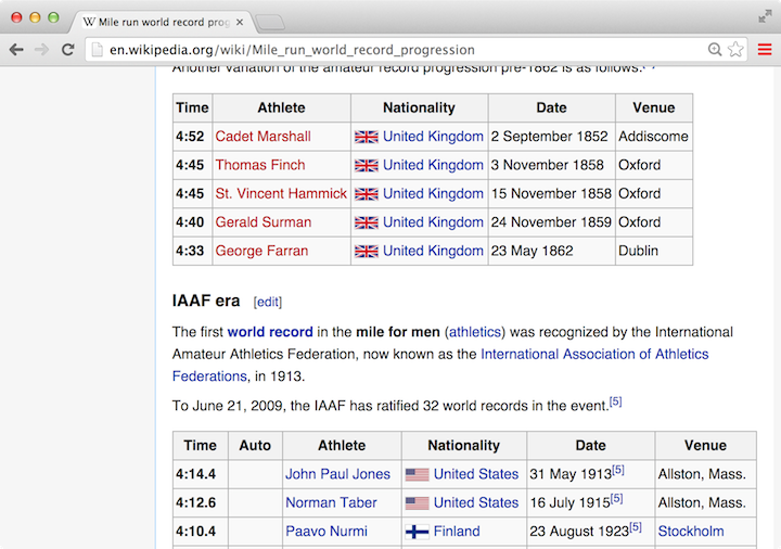
When you have the URL of a page containing one or more tables, it is sometimes easy to read them in to R as data frames. Rather than using a CSV file-reading function like fread(), use the general purpose read_html(). Once you have the content of the web page, you can translate any tables in the page from HTML to data frame format.
library(rvest)
web_page <- "http://en.wikipedia.org/wiki/Mile_run_world_record_progression"
SetOfTables <- web_page %>%
  read_html() %>%
  html_nodes(css = "table") %>%
  html_table(fill = TRUE)
The result, SetOfTables, is not a data frame. Instead, it is a list A list is an R object used to store a collection of other R objects. Elements of a list can even have different types–e.g., data frames, plots, model objects, even other lists. of the tables found in the web page. Use length() to find how many items there are in the list of tables.
## [1] 12You can access any of those 12 tables. The first table is SetOfTables[[1]], the second table is SetOfTables[[2]], and so on. Note the use of double square brackets. As it happens, the tables shown in Figure 16.1 are the third and fourth in the running-records web page at the time of this writing. Of course, Wikipedia pages are subject to change at any time.
Table 16.3: A data frame representing the third table embedded in the Wikipedia page on running records.
| Time | Athlete | Nationality | Date | Venue |
|---|---|---|---|---|
| 4:52 | Cadet Marshall | United Kingdom | 2 September 1852 | Addiscome |
| 4:45 | Thomas Finch | United Kingdom | 3 November 1858 | Oxford |
| 4:45 | St. Vincent Hammick | United Kingdom | 15 November 1858 | Oxford |
| 4:40 | Gerald Surman | United Kingdom | 24 November 1859 | Oxford |
| 4:33 | George Farran | United Kingdom | 23 May 1862 | Dublin |
Table 16.4: A data frame representing the fourth table embedded in the Wikipedia page on running records.
| Time | Auto | Athlete | Nationality | Date | Venue |
|---|---|---|---|---|---|
| 4:14.4 | John Paul Jones | United States | 31 May 1913[6] | Allston, Mass. | |
| 4:12.6 | Norman Taber | United States | 16 July 1915[6] | Allston, Mass. | |
| 4:10.4 | Paavo Nurmi | Finland | 23 August 1923[6] | Stockholm | |
| 4:09.2 | Jules Ladoumègue | France | 4 October 1931[6] | Paris | |
| 4:07.6 | Jack Lovelock | New Zealand | 15 July 1933[6] | Princeton, N.J. | |
| 4:06.8 | Glenn Cunningham | United States | 16 June 1934[6] | Princeton, N.J. | |
| … and so on for 32 rows altogether. |
Of course, you might prefer to use names that are more descriptive than Table3 and Table4.
16.4 Cleaning Data
A person somewhat knowledgeable about running would have little trouble interpreting the Tables 16.3 and 16.4 correctly. The Time is in minutes and seconds. The Date gives the day on which the record was set. But when the data set is read into R, both Time and Date are stored as character strings. Before they can be used, they have to be converted into a format that the computer can process like a date and time. Among other things, this requires dealing with the [5] at the end of the Date information which had represented a footnote citation on the original Wikipedia page.
Data cleaning refers to taking the information contained in a variable and transforming it to a form in which that information can be used.
16.4.1 Recoding
Table 16.5 displays a few variables from Table 16.2 describing 1728 houses houses for sale in Saratoga, NY.1 The example comes from Prof. Richard DeVeaux at Williams College. The full table includes additional variables such as living_area, price, bedrooms, and bathrooms. The data on house systems, such as sewer type and heat type have been stored as numbers, even though they are really categorical.
Houses <-
  read_csv("https://mdbeckman.github.io/dcSupplement/data/houses-for-sale.csv")

Houses %>%
  select(fuel, heat, sewer, construction)
Table 16.5: Four of the variables from the houses-for-sale.csv file giving features of the Saratoga, NY houses stored as integer codes. Each case is a different house.
| fuel | heat | sewer | construction |
|---|---|---|---|
| 3 | 4 | 2 | 0 |
| 2 | 3 | 2 | 0 |
| 2 | 3 | 3 | 0 |
| 2 | 2 | 2 | 0 |
| 2 | 2 | 3 | 1 |
| 2 | 2 | 2 | 0 |
| … and so on for 1,728 rows altogether. |
There’s nothing fundamentally wrong with using integers to encode something like fuel type, but it can be confusing to interpret results. Worse, the numbers imply a meaningful order to the categories when there is none.
To translate the integers to a more informative coding, you first have to find out what the various codes mean. Often, this information comes from the codebook, but sometimes you will need to contact the person who collected the data.
Once you know the translation, you can use spreadsheet software to enter them into a data frame, like this one for the houses:
Table 16.6: Codes for the house system types found in the Translations data.
| code | system_type | meaning |
|---|---|---|
| 0 | new_const | no |
| 1 | new_const | yes |
| 1 | sewer_type | none |
| 2 | sewer_type | private |
| 3 | sewer_type | public |
| 0 | central_air | no |
| … and so on for 13 rows altogether. |
Translations describes the codes in a format that makes it easy to add new code values as the need arises. The same information can also be presented a wide format as in Table 16.7.
Table 16.7: The CodeVals data frame: Translations rendered in a wide format.
| code | central_air | fuel_type | heat_type | new_const | sewer_type |
|---|---|---|---|---|---|
| 0 | no | invalid | invalid | no | invalid |
| 1 | yes | invalid | invalid | yes | none |
| 2 | invalid | gas | hot air | invalid | private |
| 3 | invalid | electric | hot water | invalid | public |
| 4 | invalid | oil | electric | invalid | invalid |
In CodeVals, there is a column for each system type that translates the integer code to a meaningful term. In cases where the integer has no corresponding term, invalid has been entered. This provides a quick way to distinguish between incorrect entries and missing entries.
To carry out the translation, join each variable, one at a time, to the data frame of interest. Note how the by value changes for each variable:
Houses <-
  Houses %>%
  left_join(CodeVals %>% select(code, fuel_type),
            by = c(fuel = "code")) %>%
  left_join(CodeVals %>% select(code, heat_type),
            by = c(heat = "code")) %>%
  left_join(CodeVals %>% select(code, sewer_type),
            by = c(sewer = "code"))
Table 16.8 shows the re-coded data.
Table 16.8: The Houses data with re-coded categorical variables.
| fuel_type | heat_type | sewer_type |
|---|---|---|
| electric | electric | private |
| gas | hot water | private |
| gas | hot water | public |
| gas | hot air | private |
| gas | hot air | public |
| gas | hot air | private |
| … and so on for 1,728 rows altogether. |
16.4.2 From Strings to Numbers
You’ve seen two major types of variables: quantitative and categorical. You’re used to using quoted character strings as the levels of categorical variables, and numbers for quantitative variable.
Often, you will encounter data frames that have variables whose meaning is numeric but whose representation is a character string. This can occur when one or more cases is given a non-numeric value, e.g., not available.
The as.numeric() function will translate character strings with numerical content into numbers. as.character() goes the other way.
For example, in the OrdwayBirds data, the Month, Day and Year variables are all being stored as character string, even though their evident meaning is numeric. Convert the strings to numbers like this:
OrdwayBirds <-
  OrdwayBirds %>%
  mutate(Month = as.numeric(Month),
         Year = as.numeric(Year),
         Day = as.numeric(Day))
If the numerical strings have punctuation, e.g. "¥2,540,937", the readr::parse_number() function is effective.
16.4.3 Dates
Dates are generally written down as character strings, for instance, “29 October 2014”. Dates have a natural order. When you plot values such as 16 December 2017 and 29 October 2016, you expect the December date to come after the October date, even though this is not true alphabetically of the string itself.
When plotting a value that is numeric, you expect the axis to be marked with a few round numbers. A plot from 0 to 100 might have ticks at 0, 20, 40, 60, 100. It’s similar for dates. When you are plotting dates within one month, you expect the day of the month to be shown on the axis. But if you are plotting a range of several years, you it would be appropriate to show only the years on the axis.
When you are given dates stored as a character string, it can be useful to convert them to a computer format designed specifically for dates. For instance, in the OrdwayBirds data, the Timestamp variable refers to the time the data were transcribed from the original lab notebook to the computer file. You can translate the character string into a genuine date using functions from the lubridate package. Table 16.9 shows a few of the date character strings from the Timestamp variable in OrdwayBirds.
Table 16.9: A few timestamp strings from OrdwayBirds.
| Timestamp |
|---|
| 2/24/2011 10:43:03 |
| 11/8/2010 17:00:34 |
| 2/16/2012 10:27:54 |
These dates are written in a format showing month/day/year hour:minute:second. The mdy_hms() function from the lubridate package converts strings in this format to a date. As an example, suppose you want to examine when the entries were transcribed and who did them. You might create a data frame and plot, as in Table ?? and Figure 16.2 as shown.
library( lubridate )

WhenAndWho <-
  OrdwayBirds %>%
  select(Who = DataEntryPerson, When = Timestamp) %>%
  mutate(When = mdy_hms(When))
Table 16.10: WhenAndWho: The times at which OrdwayBirds data were transcribed.
| Who | When |
|---|---|
| Jerald Dosch | 2010-04-14 13:20:56 |
| Caitlin Baker | 2010-05-13 16:00:30 |
| Caitlin Baker | 2010-05-13 16:02:15 |
| Caitlin Baker | 2010-05-13 16:03:18 |
| Caitlin Baker | 2010-05-13 16:04:23 |
| Caitlin Baker | 2010-05-13 16:06:15 |
| … and so on for 15,825 rows altogether. |
Figure 16.2: The transcribers of OrdwayBirds from lab notebooks worked at different times of day.
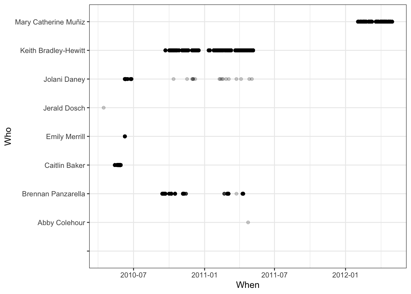
Many of the same operations that apply to numbers can be used on dates. For example, Table 16.11 displays the date range worked by various transcribers calculated as a difference in times.
WhenAndWho %>%
  group_by(Who) %>%
  summarise(start = min(When, na.rm=TRUE),
            finish = max(When, na.rm=TRUE))
Table 16.11: Starting and ending dates for each transcriber involved in the OrdwayBirds project.}
| Who | start | finish |
|---|---|---|
| Abby Colehour | 2011-04-23 | 2011-04-23 |
| Brennan Panzarella | 2010-09-13 | 2011-04-10 |
| Caitlin Baker | 2010-05-13 | 2010-05-28 |
| … and so on for 8 rows altogether. |
There are many similar lubridate functions for converting into dates strings in different formats, e.g. ymd(), dmy(), and so on. There are also functions like hour(), yday(), etc.
16.5 Factors or Strings?
R was designed with a special type for holding categorical data: “factors”. Factors store categorical data efficiently and provide a means to put the categorical levels in whatever order is desired. Unfortunately, factors also make cleaning data more confusing. The problem is that it’s easy to mistake a factor for a character string, but they have different properties when it comes to conversion to numeric or date form and especially when using the character processing techniques in Chapter 17.
By default, readr::read_csv(), data.table::fread(), and mosaic::read.file() will interpret character strings as just that. Other functions such as read.csv() convert character strings into factors by default. Cleaning such data often requires converting it back to character-string format using as.character(). Failing to do this when needed can result in completely erroneous results without any warning.
For this reason, the data sets used in this book have been stored with categorical or text data in character-string format. Be aware that data provided by other packages do not necessarily follow this convention. So, if you get mysterious results when working with such data, consider the possibility that you are working with factors rather than character strings.
CSV files in this book are typically read with read_csv(). If, for some reason, you prefer to use the read.csv() function, make sure to specify the argument stringsAsFactors = FALSE to insist that text data be stored as character strings.
16.6 Exercises
Problem 16.1: Here are some character strings containing times or dates written in different formats. Your task is two-fold: (A) for each, choose an appropriate function from the lubridate package to translate the character string into a date-time object in R and then (B) use R to calculate the number of days between that date and your birthday.
"April 30, 1777"Johann Carl Friedrich Gauss"06-23-1912"Alan Turing’s birthday"3 March 1847"Alexander Graham Bell’s birthday"Nov. 11th, 1918 at 11:00 am"Armistice ending World War I on the Western Front."July 20, 1969"First manned moon landing
Example code:
## Time difference of 9897 daysProblem 16.2: Here are some strings containing numerical amounts. For each one, say whether as.numeric() or readr::parse_number() (or both or neither) properly converts the given string to a numeric value.
"42,659.30""17%""Nineteen""£100""9.8 m/seconds-square""9.8 m/s^2""6.62606957 × 10^-34 m2 kg / s""6.62606957e-34""42.659,30"(A European style)
Problem 16.3: Grab Table 4 (or another similar table) from the Wikipedia page on world records in the mile (or some similar event). Make a plot of the record time versus the date in which it occurred. Also, mark each point with the name of the athlete written above the point. (Hint: Use geom_text())
Some Tips:
To convert time entries such as “4:20.5” into seconds, use the
lubridatepackage’sas.duration(ms("4:20.5")).You can get rid of the footnote markers such as
[5]in the dates with a statement like this:
- The
gsub()transformation function replaces the characters identified in the first argument with those in the second argument. The string"\\[.\\]$"is an example of a “regular expression” which identifies a pattern of characters, in this case a single character in square brackets just before the end of the string.