Chapter 4 Files and documents
In your work with data, you will be using and creating computer files of various sorts. Of particular importance are three basic roles for files:
- storing data tables
- listing R instructions
- writing reports with narrative, graphics and conclusions
Different file types are used for each of these roles. These types can be referred to by the filename extension of the files.
Table 4.1: Common file types and their uses
| File Role | Common File types | Software |
|---|---|---|
| Data storage |
.csv, .xlsx, etc.
|
Spreadsheets |
| R instructions |
.Rmd
|
Text editor, compiler |
| End reports |
.html, .pdf, .docx, etc.
|
web browser, word processor |
4.1 Filename Extensions
The filename extension is one or more letters following the last period in the name: .xlsx, .docx, .html, .mpeg. (Other widely used extensions are .pdf, .zip, .png.) These letters indicate the format of the file and often set which program will be used to open the file: a spreadsheet, a word processor, a browser, or a music player in the examples. Or, in plainer language, the filename extension tells you the kind of file.
If you are looking at files through RStudio, the filename extension will always be displayed. If you are using your your own computer’s file browser, your system may have been set up to hide the extension.
When referring to files within R statements or an Rmd file, you must always include the filename extension.
4.2 Paths
A filename is analogous to a person’s first name. Just as first names are unique within a nuclear family, so filenames must be unique within a folder or directory.To run on with the family metaphor … You are identified within a household by your first name. The path would tell you which specific nuclear family you belong to, perhaps in the form of your address, like this: USA/Saint Paul/55105/703 Lincoln Avenue.
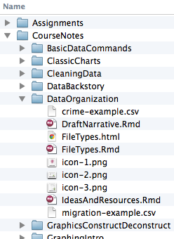
You are probably used to seeing folders and the files they contain organized on your computer as in Figure 4.1. The is the set of successive folders that bring you to the file.
Figure 4.1: Folders contained within folders, as shown by a file browser on Apple OS-X.
There is a standard format for file paths. An example:
/Users/kaplan/Downloads/0021_001.pdf
Here the filename is 0021_001, the filename extension is .pdf, and the file itself is in the Downloads folder contained in the kaplan folder, which is in turn contained in the Users folder. The starting / means “on this computer”.
The R file.choose() — which should be used only in the console, not in an Rmd file — brings up an interactive file browser. You can select a file with the browser. The returned value will be a quoted character string with the path name.
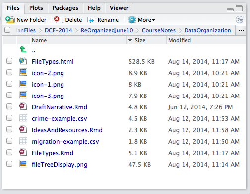
## [1] "/Users/kaplan/Downloads/0021_001.pdf"In RStudio, the Files tab will display the path near the top. In Figure 4.2, the ten files lised are all in the same folder, whose path ends with DCF-2014/ReOrganizedJune10/CourseNotes/DataOrganization.
Figure 4.2: Filenames and their file path shown in the Files tab in RStudio. Only part of the path is shown: the folders closest to the files.
Quotes or not for a file path? When you are referring to a file path in R, it will always be in quotation marks; it’s a character string. Other software such as web browsers don’t use quotes when specifying a path.
4.3 URLs
You have probably noticed URLs in the locator window near the top of your browser. In Figure , the URL is:
http://tiny.cc/dcf/index.html.
Figure 4.3: A browser directed to a website for the (print) first edition of this book at the URL http://tiny.cc/dcf/index.html
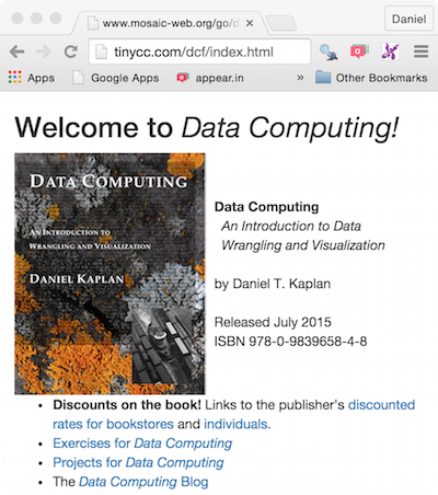
A URL includes in its path name the location of the server on which the file is stored (e.g. tiny.cc) followed by the path to the file on that server. Here, the path is /dcf and the file is index.html.
You will sometimes need to copy URLs into your work in R, to access a dataset, to make a link to some reference, etc. Remember to copy the entire URL, including the http:// part if it is there.
Some common filename extensions for the sort of web resources you will be using:
.pngfor pictures.jpgor.jpegfor photographs.csvor.Rdatafor data files.Rmdfor the human editable text of a document.htmlfor web pages themselves
4.4 Data Files
Data frames are often stored individually as files. There are many formats for data files. Among the most common is the .csv spreadsheet format, popular because reading it is a standard feature of many data analysis packages (including R).
If you use R extensively, you will also encounter data in .Rda (or .rda, or .Rdata), an efficient format for storing data and other information specifically for R. When you get data from an R package, like this:
you are in fact reading in an .Rda file associated with the package.
There are many other formats for files containing data tables or the information needed to put the contents in data-table format. These are discussed in Chapter 16. Increasingly, data are accessed through database systems. In such a case, rather than reading the database as a whole, you make “queries” to access specific data you need.
Files containing data tables are often distributed via the web. These files are not any different than files on your own computer. You access such files through a Uniform Resource Locator, better known as a URL. For instance, several supplemental data sets accompanying the Data Computing are stored as .csv files, which can be accessed directly with R commands like this:
| Engine | mass | ncylinder | strokes | displacement | bore | stroke | BHP | RPM |
|---|---|---|---|---|---|---|---|---|
| Webra Speedy | 0.135 | 1 | 2 | 1.8 | 13.5 | 12.5 | 0.45 | 22000 |
| Motori Cipolla | 0.150 | 1 | 2 | 2.5 | 15.0 | 14.0 | 1.00 | 26000 |
| Webra Speed 20 | 0.250 | 1 | 2 | 3.4 | 16.5 | 16.0 | 0.78 | 22000 |
| Webra 40 | 0.270 | 1 | 2 | 6.5 | 21.0 | 19.0 | 0.96 | 15500 |
| Webra 61 Blackhead | 0.430 | 1 | 2 | 10.0 | 24.0 | 22.0 | 1.55 | 14000 |
| Webra 6WR | 0.490 | 1 | 2 | 10.0 | 24.0 | 22.0 | 2.76 | 19000 |
| … and so on for 39 rows altogether. |
So far as accessing data is concerned, there’s nothing fundamentally different in reading a file from a URL than reading a file on your own computer.
4.5 Documenting your work with Rmd files
The purpose of data wrangling and visualization is communication: condensing and presenting data in a form that conveys information. An important part of communication is documentation and reporting.
Writing is not a linear process. Ideas are presented, revised or abandoned, corrected, re-focussed, and re-arranged. Data-oriented technical reports tie together narrative, graphics and summary tables and are based on potentially complex computer commands. There is an interplay between the computer commands and the narrative. Results from the computer may drive reconsideration of the narrative. Gaps in the narrative may point to shortcomings or omissions in the computer commands. And, always, there is the possibility of errors in writing commands and the need to document commands so that they can be checked and corrected. As well, data are commonly updated, corrected or extended.
The familiar practice of cutting and pasting from the computer console into a word processor does not address these features of technical reports. Cutting and pasting makes it hard to revise or update a report; you’ve got to cut out the old and paste in the new, figuring out for yourself which is which. This introduces the likelihood of error. And, there’s nothing to document the linkages between the computer commands and the word-processed document.
An important concept in data-driven reporting is reproducibility. The idea is to be able to reproduce your entire document without any manual intervention, and, more important, to be easily able to generate a new report in response to changes in data or revisions in computer commands. In other words, reproducible reports contain all the information needed to generate a new report. Common document formats such as .pdf, .docx, or .html do not offer support for reproducibility.
In R, reproducible reporting is provided by the .Rmd file format and related software. An .Rmd file integrates computer commands into the narrative so that, for instance, graphics are produced by the commands rather than being inserted from another source.
You create and modify reproducible reports within RStudio’s text editor. An .Rmd file contains ordinary text and punctuation: no formatting, color, imagesIn fact, R Notebook functionality may allow the user to see an embedded preview of images, R output, etc in the RStudio environment. The .Rmd is technically just the text file., etc. Instead, you use the .Rmd file to describe, using ordinary characters, both what you want the eventual format to look like and what R commands you want the computer to carry out in generating the report.
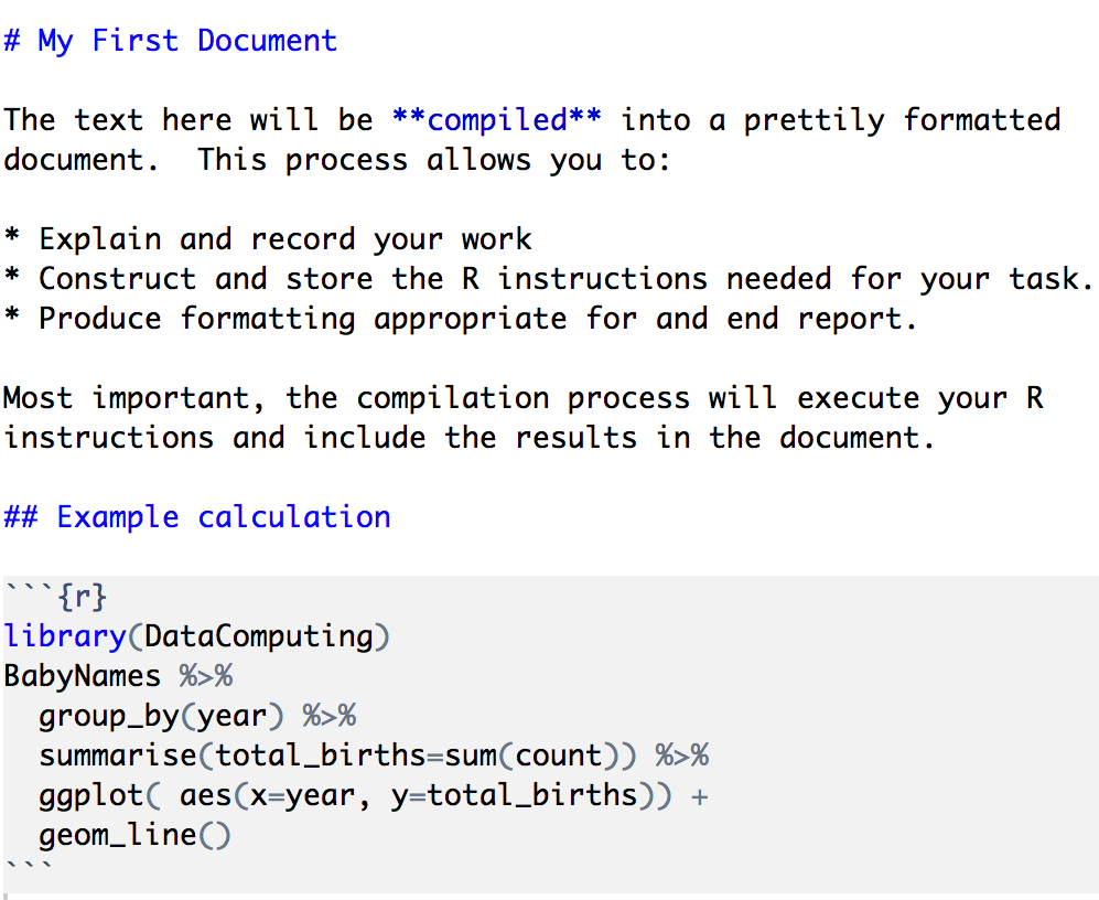
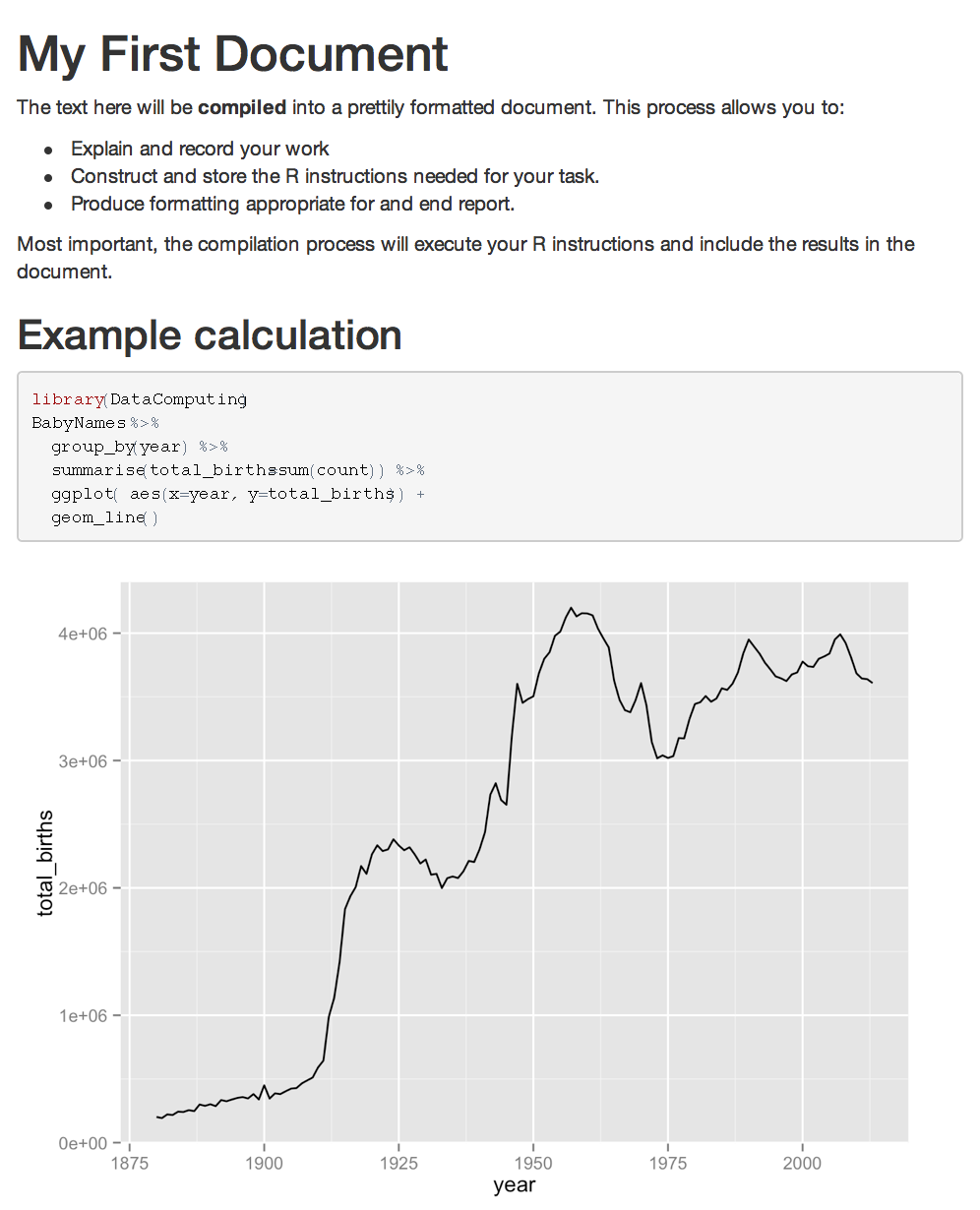
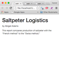
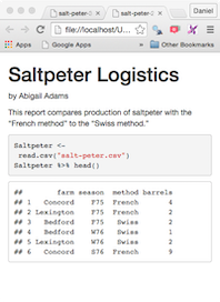
Figure 4.4 shows a simple .Rmd document, something you might write. The figure also shows the .html file that is the result of compiling the .Rmd.
Figure 4.4: The .Rmd file on consists of plain text that is automatically compiled to the formatted .html document, with the results of calculations.
4.6 The Write/Compile Cycle
After you edit an .Rmd file, you compile the report into a reader-friendly document format such as .pdf, .docx, or .html that can easily be printed or displayed on the report-reader’s computer. You never edit the reader-friendly document; it’s created automatically from your .Rmd instructions. When you want to update or modify or correct the end report, you edit the .Rmd file and then recompile to produce the updated version of the corresponding reader-friendly document.
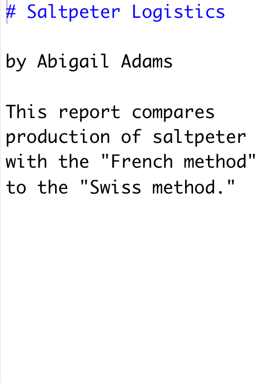
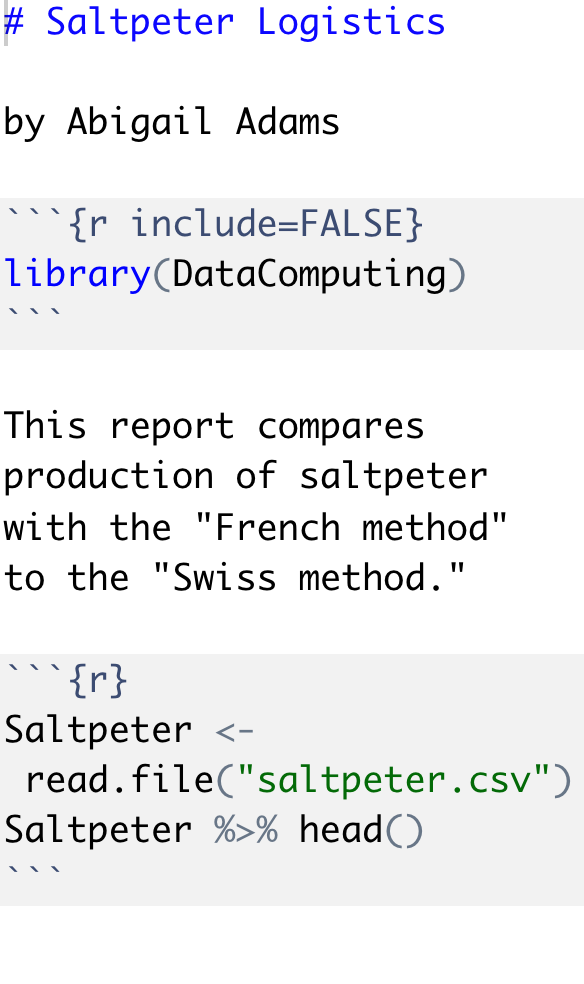
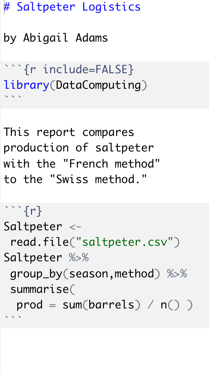
It’s a good strategy to compile your .Rmd frequently. Start with a small, simple document. Then add a bit more to it: one paragraph or one “chunk” (see below). Compile again. If something goes wrong, you will have a good idea of where the problem lies. Go back and fix things. Make small changes, compile, see if it worked. Repeat. Figure 4.5 shows several steps in such an editing cycle.
| Step 1. Start with a short and simple document | Step 2. Add the boilerplate chunk and a chunk to your start your wrangling. Test that it works. If not, go back and fix it. | Step 3. Add more to the wrangling chunk. Test that it works. |
|---|---|---|
 |
 |
 |
| Compile to HTML | Compile to HTML | Compile to HTML |
 |
 |
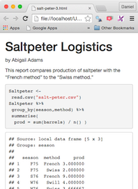 |
Figure 4.5: Three steps in the write/compile cycle. At each step, the .Rmd file (shown in monospace font) is compiled into the .html format shown underneath.

It’s impossible to avoid errors; even professionals make them. Instead, adopt a process that let’s you identify errors quickly so that you can fix them before moving on. The shorter the write/compile cycle, the easier it will be to know when you have erred.
4.7 Command Chunks
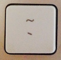
The R commands in an .Rmd file go into chunks, a range of lines in the documents that are delimited in a special way so that they will be executed as part of the .Rmd \(\rightarrow\) .html compilation process.1 Exactly the same applies when compiling to .pdf or .docx. The opening delimiter is ```{r}. The closing delimiter is simply ```. Both the opening and closing delimiters for a chunk are “back-quotes,” a quote character that goes from upper-left to bottom-right. On many keyboards, back-quote is on the same key as tilde ~, like this:
 For example:
```{r}
Saltpeter <- read_csv("https://mdbeckman.github.io/dcSupplement/data/saltpeter.csv")
```
Most .Rmd files will draw on a library that needs to be loaded into the R session. When you compile .Rmd \(\rightarrow\) .html, R starts a brand new session that is, initially, empty and with no libraries loaded. When the compilation is complete, that session evaporates, leaving as its only residue the .html result.Because R starts a brand new session in this way, interactive commands such as file.choose() cannot be used in an an .Rmd file; there’s no opportunity for any user to interact during the automatic compilation process. Instead, use the interactive command in the console, get the result, and paste that result into your .Rmd file.
Often, the first chunk in your document will be an instruction to load one or more libraries. Since this will be in just about every .Rmd document, it can be called the boilerplate chunk. It looks like this:
```{r include=FALSE}
library(dcData)
# and any others that you need, e.g.
library(tidyverse)
library(mosaic)
```
A boilerplate chunk goes at the start of the document. It loads the libraries that the following commands will use.
The include=FALSE chunk argument helps to prettify the document: it is an instruction not to show the contents of the chunk in the output file.
Distributing the .Rmd file is helpful when communicating with a technically savvy audience. A nice strategy for getting the benefits of both the easily-readable .html format and the original .Rmd file is to include the .Rmd file inside the .html, much as you might attach a file to an email message. R Notebook functionality in RStudio embeds the source .Rmd file automatically. The resulting file has extension .nb.html. but functions in all other ways as a typical .html file should.
4.8 Exercises
Problem 4.1: Markdown provides a simple way to produce section headers and sub-headers, italic and bold text, monospaced fonts suitable for computer commands, and even web links. A reference is available in RStudio at the menu Help/Markdown Quick Reference.
For each of the following, say how it will be rendered when the Markdown is rendered to HTML. (Hint: You can figure it out by reading the documentation, or you can put the text into an Rmd document and compile it!)
*one***two*** three# Four`five`## Six[seven](https://www.r-project.org/)
Problem 4.2: What’s wrong with the markup for each of these five chunks:
Problem 4.3: Treat the following lines as an .Rmd file which will be compiled to HTML.
### An Introduction

Arithmetic is *easy*! For instance
```{r}
3 + 2
```
Using paper and pencil, sketch out what the HTML document will look like when viewed in a web browser.
Problem 4.4: Here is a short list of names:
DataComputing.orgahab/whale.Rmdptth://world-bank.orghttp://world-bank.org//world-bank.org/index.htmlworld-bank.org/index.html
For each, say whether the name is in the allowed form for a possible URL, a possible file, neither, or both.
Problem 4.5: Here are several possibilities for file content:
- Formatted document content
- Image (Photo or Non-photo)
- Specification of the contents of a document
- Spreadsheet or data table contents
- A what-you-see-is-what-you-get document
For each of the following filename extensions, indicate the sort of content (from the numbered list above) associated with the extension.
.csv.Rmd.jpg.Rdata.docx.html.ppt.png.txt.xlsx