Chapter 1 Tidy Data
Data can be as simple as a column of numbers in a spreadsheet file or as complex as the medical records collected by a hospital. A newcomer to working with data may expect each source of data to be organized in a unique way and to require unique techniques. The expert, however, has learned to operate with a small, standard set of tools. As you’ll see, each of the standard tools performs a comparatively simple task. Combining those simple tasks in appropriate ways is the key to dealing with complex data.
One reason the individual tools can be simple is this: each tool gets applied to data arranged in a simple but precisely defined pattern called tidy data. At the heart of tidy data is the data table. To illustrate, Table 1.1 contains a handful of entries from a large US Social Security Administration tabulation of names given to babies. In particular, the table shows how many babies of each sex were given each name in each year.
Table 1.1: A data frame showing how many babies were given each name in each year in the US.
| name | sex | count | year |
|---|---|---|---|
| Sherina | F | 19 | 1970 |
| Leketha | F | 6 | 1973 |
| Tahirih | F | 6 | 1976 |
| Radha | F | 13 | 1979 |
| Hatim | M | 8 | 1981 |
| Cissy | F | 7 | 1984 |
| Ahmet | M | 6 | 1986 |
| … and so on for 1,792,091 rows altogether. |
Table 1.1 shows there were 6 boys named Ahmet born in the US in 1986 and 19 girls named Sherina born in 1970. As a whole, the BabyNames data table covers the years 1880 through 2013 and includes a total of 333,417,770 individuals, somewhat larger than the current population of the US.
The data in Table 1.1 are “tidy” because they are organized according to two simple rules.
- The rows, called cases, each refer to a specific, unique and similar unit of observation, e.g. girls named Sherina in 1970.
- The columns, called variables, each refer a specific attribute, feature, or measurement of the cases. For instance,
countgives the number of babies for each case;sexindicates if the case is male (M) of female (F).
When data are in tidy form, it’s often straightforward to transform the data into arrangements that are useful for answering interesting questions. For instance, you might wish to know which were the most popular baby names over all the years. Even though Table 1.1 contains the popularity information implicitly, some re-arrangement is needed (for instance, adding up the counts for a name across all the years) before the information is made explicit, as in Table 1.2.
Table 1.2: The number of babies given each name, sorted from most to least popular.
| sex | name | total_births |
|---|---|---|
| M | James | 5091189 |
| M | John | 5073958 |
| M | Robert | 4789776 |
| M | Michael | 4293460 |
| F | Mary | 4112464 |
| M | William | 4038447 |
| … and so on for 102,690 rows altogether. |
The process of transforming information that is implicit in a data table into another data table that gives the information explicitly is called data wrangling. The wrangling itself is accomplished by using data verbs that take a tidy data table and transform it into another tidy data table in a different form. In the following chapters, you will be introduced to the various data verbs.
1.1 Rules for tidy data
Being neat is not what makes data tidy. For instance, consider the spreadsheet shown in Figure 1.1. The spreadsheet is not in tidy form. True, the spreadsheet is attractive and neatly laid out. There are helpful labels and summaries that make it easy for a person to read and draw conclusions. For instance, Ward 1 had a higher voter turnout than Ward 2, and both wards were lower than the city total.
Figure 1.1: A spreadsheet showing ward and precinct votes cast in the 2013 Minneapolis mayoral election.
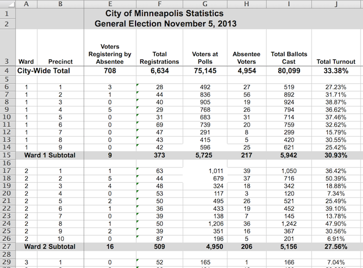
However neat it is, the spreadsheet in Figure 1.1 violates the rules for tidy data.
Rule 1: The rows, called cases, each must represent the same underlying attribute, that is, the same kind of thing.
That’s not true in Figure 1.1. For most of the spreadsheet, the rows represent a single precinct. But other rows give ward or city-wide totals. The first two rows are captions describing the data, not cases.
Rule 2: Each column is a variable containing the same type of value for each case.
That’s mostly true in Figure 1.1, but the tidy pattern is interrupted by labels that are not variables. For instance, the first two cells in row 15 are the label “Ward 1 Subtotal,” different from the ward/precinct identifiers that are the values in most of the first column.
Conforming to the rules for tidy data simplifies summarizing and analyzing data. For instance, in the tidy baby names table, it’s easy to find the total number of babies: just add up all the numbers in the count variable. It’s similarly easy to find the number of cases: just count the rows. And if you want to know the total number of Ahmeds or Sherinas across the years, there’s an easy way to do that.
In contrast, it would be more difficult in the Minneapolis election data to find, say, the total number of ballots cast. If you take the seemingly obvious approach and add up the numbers in column I of the spreadsheet in Figure 1.1 (labelled “Total ballots cast”), the result will be three times the true number of ballots, because some of the rows contain summaries, not cases.
Indeed, if you wanted to do calculations based on the Minneapolis election data, you would be far better off to put it in a tidy form, like Table 1.3.
Table 1.3: The Minneapolis election data in tidy form.
| ward | precinct | registered | voters | absentee | total.turnout |
|---|---|---|---|---|---|
| 1 | 1 | 28 | 492 | 27 | 0.2723 |
| 1 | 4 | 29 | 768 | 26 | 0.3662 |
| 1 | 7 | 47 | 291 | 8 | 0.1579 |
| 2 | 1 | 63 | 1011 | 39 | 0.3642 |
| 2 | 4 | 53 | 117 | 3 | 0.0734 |
| 2 | 7 | 39 | 138 | 7 | 0.1378 |
| … and so on for 117 rows altogether. |
The tidy form is, admittedly, not as attractive as the form published by the Minneapolis government. But the tidy form is much easier to use for the purpose of generating summaries and analyses.
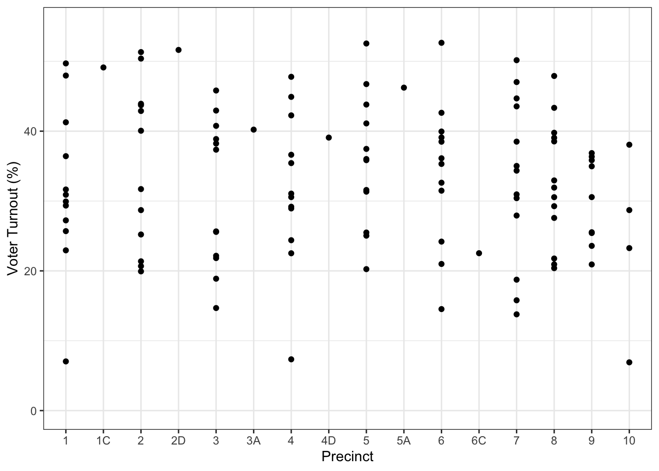
Once data are in a tidy form, you can present them in ways that can be more effective than a formatted spreadsheet. Figure 1.2 presents the turnout in each ward that makes it easy to see how much variation there is within and among precincts.
Figure 1.2: A graphical depiction of voter turnout in the different wards.
The tidy format also makes it easier to bring together data from different sources. For instance, to explain the variation in voter turnout, you might want to look at variables such as party affiliation, age, income, etc. Such data might be available on a ward-by-ward basis from other records, such as the (public) voter registration logs and census records. Tidy data can be recast, summarized, combined, or otherwise wrangled into forms that make it more suitable for a given purpose. This would be difficult if you had to deal with an idiosyncratic format for each different source of data.
1.2 Variables
In data science, the word variable has a different meaning than in mathematics. In algebra, a variable is an unknown quantity. In data, a variable is known; it represents a feature that has been measured or observed. “Variable” refers to a specific quantity or quality that can vary from one case to another.
There are two major types of variables: quantitative and categorical. A quantitative variable is just what it sounds like: a number.
A categorical variable tells which category or group a case falls into. For instance, in the baby names data table, sex is a categorical variable with two levels, F and M, standing for female and male. Similarly the name variable is categorical. It happens that there are 92,600 different levels for name, ranging from Aaron, Ab, and Abbie to Zyhaire, Zylis, and Zymya.
1.3 Cases and what they represent
As already stated, a row of a tidy data table refers to a case. To this point, you may have little reason to prefer the word case to row. .
When working with a data table, it’s important to keep in mind what a case stands for in the real world. Sometimes the meaning is obvious. For instance, Table 1.4 is a tidy data table showing the ballots in the Minneapolis mayoral election in 2013. Each case is an individual voter’s ballot. (The voters were directed to mark their ballot with their first choice, second choice and third choice among the candidates. This is part of a procedure called rank choice voting: See http://vote.minneapolismn.gov/rcv/.)
Table 1.4: Individual ballots in the Minneapolis election. Each voter votes in one ward in one precinct. The ballot marks the voter’s first three choices for mayor.
| Precinct | First | Second | Third | Ward |
|---|---|---|---|---|
| P-10 | BETSY HODGES | undervote | undervote | W-7 |
| P-06 | BOB FINE | MARK ANDREW | undervote | W-10 |
| P-09 | KURTIS W. HANNA | BOB FINE | MIKE GOULD | W-10 |
| P-05 | BETSY HODGES | DON SAMUELS | undervote | W-13 |
| P-01 | DON SAMUELS | undervote | undervote | W-5 |
| P-04 | undervote | undervote | undervote | W-6 |
| … and so on for 80,101 rows altogether. |
The case in Table 1.4 is a different sort of thing than the case in Table 1.3. In Table 1.3, a case is a ward in a precinct. But in Table 1.4, the case is an individual ballot. Similarly, in the baby names data (Table 1.1), a case is a name and sex and year while in Table 1.2 the case is a name and sex.
When thinking about cases, ask this question: What description would make every case unique? In the vote summary data, a precinct does not uniquely identify a case. Each individual precinct appears in several rows. But each precinct & ward combination appears once and only once. Similarly, in Table 1.1, name & sex do not specify a unique case. Rather, you need the combination of name & sex & year to identify a unique row.
Example: Runners and Races
Table 1.5 shows some of the results from a 10-mile running race held each year in Washington, D.C.
Table 1.5: An excerpt of runners’ performance over the years in a 10-mile race.
| name.yob | sex | age | year | gun |
|---|---|---|---|---|
| jane polanek 1974 | F | 32 | 2006 | 114.50000 |
| jane poole 1948 | F | 55 | 2003 | 92.71667 |
| jane poole 1948 | F | 56 | 2004 | 87.28333 |
| jane poole 1948 | F | 57 | 2005 | 85.05000 |
| jane poole 1948 | F | 58 | 2006 | 80.75000 |
| jane poole 1948 | F | 59 | 2007 | 78.53333 |
| jane schultz 1964 | F | 35 | 1999 | 91.36667 |
| jane schultz 1964 | F | 37 | 2001 | 79.13333 |
| jane schultz 1964 | F | 38 | 2002 | 76.83333 |
| jane schultz 1964 | F | 39 | 2003 | 82.70000 |
| jane schultz 1964 | F | 40 | 2004 | 87.91667 |
| jane schultz 1964 | F | 41 | 2005 | 91.46667 |
| jane schultz 1964 | F | 42 | 2006 | 88.43333 |
| jane smith 1952 | F | 47 | 1999 | 90.60000 |
| jane smith 1952 | F | 49 | 2001 | 97.86667 |
What’s the meaning of a case here? It’s tempting to think that a case is a person. After all, it’s people who run road races. But notice that individuals appear more than once: Jane Poole ran each year from 2003 to 2007. (Her times improved consistently as she got older!) Jane Smith ran in the races from 1999 to 2006, missing only the year 2000 race. This suggests that the case is a runner in one year’s race.
1.4 The Codebook
Data tables do not necessarily display all the variables needed to figure out what makes each row unique. For such information, you sometimes need to look at the documentation of how the data were collected and what the variables mean.
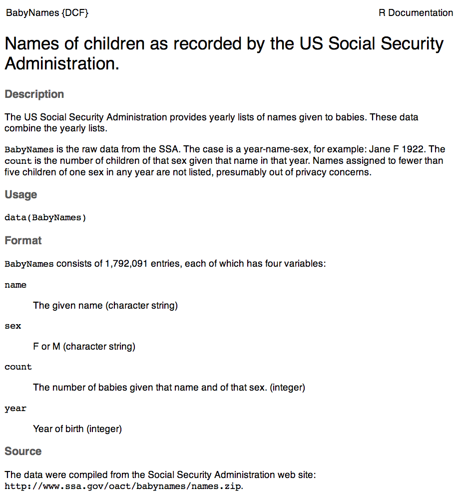
The codebook is a document — separate from the data table — that describes various aspects of how the data were collected, what the variables mean and what the different levels of categorical variables refer to. Figure 1.3 shows the codebook for the BabyNames data in Figure 1.1.
The word “codebook” comes from the days when data was encoded for the computer in ways that make it hard for a human to read. A codebook should also include information about how the data were collected and what constitutes a case.
Figure 1.3: The codebook for the BabyNames data table.
For the runners data in Table 1.5, the codebook tells you that the meaning of the gun variable is the time from when the starter’s pistol was fired at the beginning of the race to when the runner crosses the finish line and that the unit of measurement is “minutes.” It should also state what might be obvious: that age is the person’s age in years and sex has two levels, male and female, represented by M and F.
1.5 Multiple Tables
It’s often the case that creating a meaningful display of data involves combining data from different sources and about different kinds of things. For instance, you might want your analysis of the runners’ performance data in Table 1.5 to include temperature and precipitation data for each year’s race. Such weather data is likely contained in a table of daily weather measurements.
In many circumstances, there will be multiple tidy tables, each of which contains information relative to your analysis but has a different kind of thing as a case. Chapter 11 is about techniques combining data from such different tables. For now, keep in mind that being tidy is not about shoving everything into one table.
1.6 Exercises
Problem 1.1: Here is an excerpt from the baby-name data set.
| name | sex | count | year |
|---|---|---|---|
| Taffy | F | 19 | 1970 |
| Liliana | F | 162 | 1973 |
| Stan | M | 55 | 1975 |
| Nettie | F | 45 | 1978 |
| Kateria | F | 8 | 1980 |
| Nataki | F | 5 | 1982 |
| … and so on for 1,792,091 rows altogether. |
Consider these five entities, that appear in the table shown above (a) through (e):
Taffyb)yearc)sexd)namee)count
For each, choose one of the following:
- It’s a categorical variable.
- It’s a quantitative variable.
- It’s the value of a variable for a particular case.
Problem 1.2: What’s not tidy about this table?
president |
in office |
number of states |
|---|---|---|
| Lincoln, Abraham | 1861-1865 | it depends |
| George Washington | 1791-1799 | 16 |
| Martin Van Buren | 1837 to 1841 | 26 |
Re-write the table in a tidy form. Take care to render the information about years and about the number of states as numbers.
Problem 1.3: Here are three different ways of organizing the same data:
Data Table A
| Year | Algeria | Brazil | Columbia |
|---|---|---|---|
| 2000 | 7 | 12 | 16 |
| 2001 | 9 | 14 | 18 |
Data Table B
| Country | Y2000 | Y2001 |
|---|---|---|
| Algeria | 7 | 9 |
| Brazil | 12 | 14 |
| Columbia | 16 | 18 |
Data Table C
| Country | Year | Value |
|---|---|---|
| Algeria | 2000 | 7 |
| Algeria | 2001 | 9 |
| Brazil | 2000 | 12 |
| Columbia | 2001 | 18 |
| Columbia | 2000 | 16 |
| Brazil | 2001 | 14 |
- What are the variables in each table?
- What is the meaning of a case for each table? Here are some possible choices.
- A country
- A country in a year
- A year
Problem 1.4: The codebook for several data tables relating to airports, airlines, and airline flights in the US is published at https://cran.r-project.org/web/packages/nycflights13/ nycflights13.pdf.
Within that document is the codebook for the data table airports.
- How many variables are there?
- What do the cases represent?
- For each variable, make a reasonable guess about whether the values will be numerical or categorical.
Problem 1.5: In the 10-mile race data (part of which is shown below), the meaning of row-case is “a person in a year.”
Table 1.6: An excerpt of runners’ performance over the years in a 10-mile race.
| name.yob | sex | age | year | gun |
|---|---|---|---|---|
| jane polanek 1974 | F | 32 | 2006 | 114.50000 |
| jane poole 1948 | F | 55 | 2003 | 92.71667 |
| jane poole 1948 | F | 56 | 2004 | 87.28333 |
| jane poole 1948 | F | 57 | 2005 | 85.05000 |
| jane poole 1948 | F | 58 | 2006 | 80.75000 |
| jane poole 1948 | F | 59 | 2007 | 78.53333 |
| jane schultz 1964 | F | 35 | 1999 | 91.36667 |
| jane schultz 1964 | F | 37 | 2001 | 79.13333 |
| jane schultz 1964 | F | 38 | 2002 | 76.83333 |
| jane schultz 1964 | F | 39 | 2003 | 82.70000 |
| jane schultz 1964 | F | 40 | 2004 | 87.91667 |
| jane schultz 1964 | F | 41 | 2005 | 91.46667 |
| jane schultz 1964 | F | 42 | 2006 | 88.43333 |
| jane smith 1952 | F | 47 | 1999 | 90.60000 |
| jane smith 1952 | F | 49 | 2001 | 97.86667 |
| … and so on for 41,248 rows altogether. |
- Explain why
sex,age, andguntime are not part of the meaning of a row-case. - Suppose that another Jane Poole ran in the 2004 race at age 56. What additional data, not shown in the table, might be needed to distinguish between the two Jane Pooles?