Chapter 14 Graphing Networks
14.1 Vertices and edges
A network is a set of connections between objects. A network combines information about two different kinds of things:
- The objects themselves, generally called vertices Vertices: The objects that are being connected in a network. Sometimes called “nodes”.
- The connections — called edges Edge: The connections between pairs of vertices in a network – between pairs of vertices.
Figure 14.1: A network of relationships between the genes expressed in cancer cells from different people.
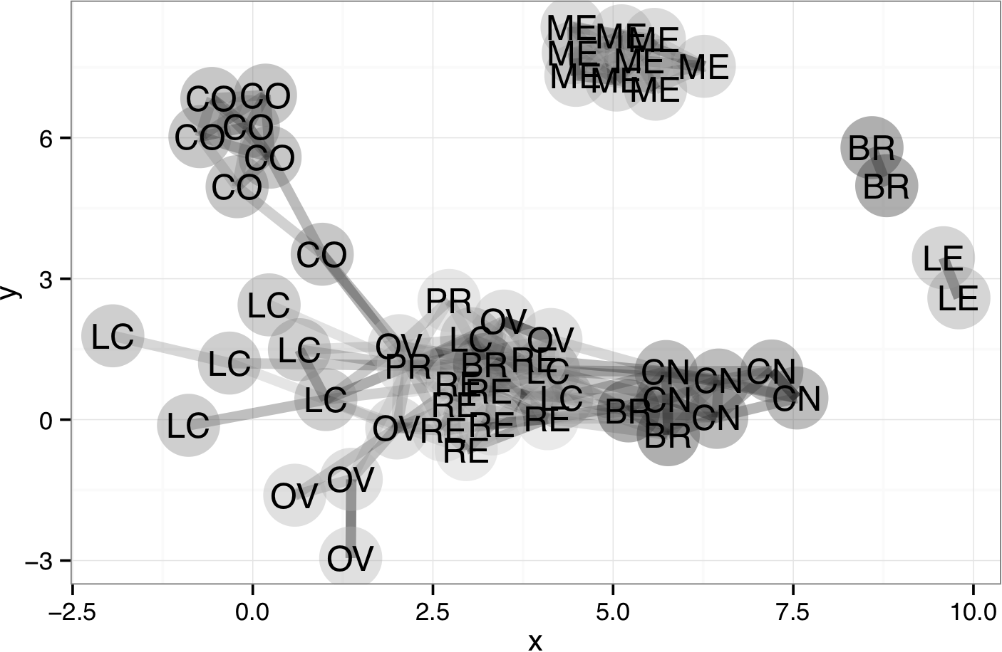
In the previous examples in this book, the end-result of data wrangling has been a single, glyph-ready data frame. With networks, things are different. A network always involves two different kinds of things — vertices and edges. Accordingly, representing a network with data always involves two different data frames:
- A data frame for the vertices, giving the properties of each vertex. In Figure 14.1 the vertices are samples of cancer cells and are shown as large dots with colors and labels identifying the type of cancer. A data frame representing the vertices might look like Table 14.1.
Table 14.1: A data frame representing the vertices in Figure 14.1.
| ID | cancerType |
|---|---|
| TK_10 | renal |
| MDA_MB_35 | melanoma |
| MCF7 | breast |
| … and so on for 60 rows altogether. |
- A different data frame for the edges. Each case in this table has at least two attributes: the origin vertex of the edge and the destination vertex of the edge. The data frame might look like Table 14.2.
Table 14.2: A data frame representing the edges in Figure 14.1.
| origin | dest |
|---|---|
| MCF7 | LOXIMV1 |
| MCF7 | UO_31 |
| LOXIMVI | HL_60 |
| SK_MEL_5 | NCI_H226 |
| SK_OV_3 | LOXIMV1 |
| HL_60 | TK_10 |
| … and so on for 241 rows altogether. |
The following sections show some of the ways that data wrangling can be used in determining what are the edges and what determines the location of each vertex in the graphic.
14.2 Example: Migration Networks
The MigrationFlows data frame presents how many people migrate between one country and another. Table 14.3 shows Bilateral, a wrangled form of MigrationFlows listing how many women migrated from one country to another and vice versa.
Table 14.3: Bilateral, which shows emigration and immigration as different variables.
| CountryA | CountryB | BtoA | AtoB |
|---|---|---|---|
| POL | DEU | 2961 | 1112903 |
| PAK | IND | 2923092 | 3995350 |
| ITA | USA | 1394 | 599174 |
| DEU | USA | 7838 | 572383 |
| GBR | CAN | 32687 | 487980 |
| IND | LKA | 15290 | 465760 |
| … and so on for 53,592 rows altogether. |
Bilateral describes edges: the links between countries. In a data frame describing edges, the case will be an edge. The minimal information needed to describe an edge is the identities of the two vertices connected by the edge.
To describe the vertices, a different data frame is required, one where each case is one vertex. The vertex data frame can contain other information about each vertex. For countries, that information might be the population or land area or GPD of each country. The glyph-ready vertex data frame should also describe where each vertex is to be located on the graph. CountryCentroids is a vertex data frame, giving the latitude and longitude of each country.
Table 14.4: CountryCentroids
| name | iso_a3 | long | lat |
|---|---|---|---|
| Afghanistan | AFG | 66.168500 | 33.78231 |
| Aland | ALA | 19.967041 | 60.19722 |
| Albania | ALB | 20.259880 | 41.14326 |
| Algeria | DZA | 2.828547 | 28.14225 |
| … and so on for 241 rows altogether. |
To show the vertices graphically, the information in the vertex data frame can be used to generate a scatter plot like Figure 14.2.
Figure 14.2: Locations of the vertices described by CountryCentroids. Another layer shows country boundaries.
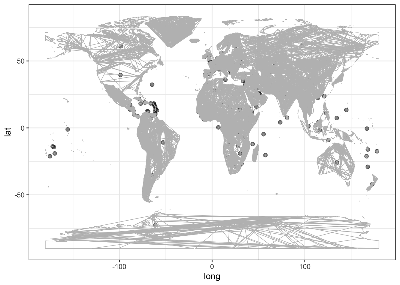
Bilateral lists the edges, which can be drawn as line segments. But Bilateral is not glyph-ready for drawing the edges. Drawing an edge requires four location attributes: x and y of the vertex at one end of the edge, and x and y of the vertex at the other end. The location of each vertex is contained in the vertex data frame, CountryCentroids. In order to wrangle Bilateral into a glyph-ready form, the location information from CountryCentroids is joined to it. This requires two join steps: joining the location of the vertex for countryA and similarly joining the location of the vertex for countryB. The result is the Edges data frame (Table 14.5).
Table 14.5: Edges, a data frame based on Bilateral wrangled into a form that is glyph-ready for drawing network edges.
| CountryA | CountryB | BtoA | AtoB | longA | latA | longB | latB |
|---|---|---|---|---|---|---|---|
| FRA | DZA | 201387 | 78867 | 2.72 | 46.53 | 2.83 | 28.14 |
| FRA | AUS | 8385 | 1925 | 2.72 | 46.53 | 134.61 | -25.85 |
| FRA | AUT | 7100 | 7460 | 2.72 | 46.53 | 14.32 | 47.60 |
| FRA | BEN | 114 | 142 | 2.72 | 46.53 | 2.55 | 9.62 |
| FRA | AND | 111 | 111 | 2.72 | 46.53 | 1.53 | 42.53 |
| FRA | AGO | 3140 | 684 | 2.72 | 46.53 | 17.74 | -12.36 |
| … and so on for 1,672 rows altogether. |
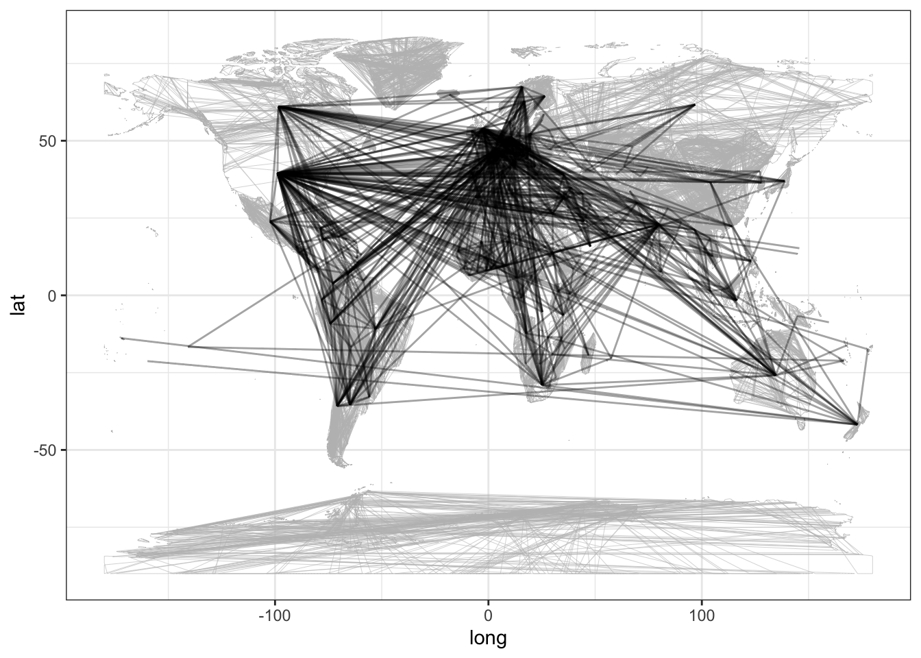
Drawing the edges can be done in the usual way. The “segment” geom is an appropriate glyph:
Figure 14.3: The edges in Bilateral using latitude and longitude to mark the location of each vertex.
14.3 Vertex Location from the Edges
It’s perfectly sensible to show the migration network using latitude and longitude for the vertex location. But many networks, for instance the gene expression network in Figure 14.1, have vertices with no natural location. Indeed, even when there is a natural location for each vertex, that might not be the best way to draw the network. Looking at Figure 14.3 critically, you can see that the graphic is dominated by the country pairs that are far apart, e.g. China and the US, Japan and Brazil, the UK and Australia. Migration among European countries, on the other hand, is compressed into a small part of the graphic. There are many crossings where the person viewing the graph can get confused.
Sometimes displays of networks are better when the vertices are placed to put them close to the vertices to which they are linked. Instead of identifying an attribute of the vertices, the location is set by the edges in a way that minimizes crossings or by some other criterion.
It’s challenging to figure out the best places for vertices to minimize the edge crossings and to keep connected vertices together. Several different methods have been described in the network-drawing literature. To simplify things, the DataComputing packageThe igraph package provides the power behind the location algorithms. provides two functions, edgesToVertices() and edgesForPlotting() to do this automatically.
To illustrate, consider a network to display cultural affinity between countries. As a simplistic measure of “cultural affinity,” use the balance between inbound and outbound migration between two countries and the number of people migrating. Here’s one way:
CulturalAffinity contains information about edges, but it has an edge even for country pairs with unbalanced migration. To show strong cultural affinity, eliminate the country pairs with unbalanced or small migration.
There are 316 edges in BigAffinity. Use edgesToVertices() to position the vertices in a way that minimizes edge crossing.
Table 14.6: Vertex location derived from CulturalAffinity using edgesToVertices().
| ID | x | y |
|---|---|---|
| FRA | -2.2706798 | 1.745457 |
| GHA | 1.6835417 | 4.868318 |
| HKG | 0.4330789 | 3.914866 |
| ISL | -5.6353426 | 5.071588 |
| AFG | -1.4635977 | -5.377435 |
| DZA | -1.8672736 | -1.541071 |
| … and so on for 125 rows altogether. |
Now that the vertex location has been determined, that location can be joined with the edge data in CulturalAffinity. This will enable the edges to be drawn connecting the vertices.
Edges <-
  Vertices %>%
  edgesForPlotting(ID = ID, x, y,
                   Edges = BigAffinity,
                   from = CountryA, to = CountryB )

Edges %>%
arrange(desc(balance))| CountryB | CountryA | BtoA | AtoB | balance | x | y | xend | yend |
|---|---|---|---|---|---|---|---|---|
| DEU | ITA | 34794 | 34918 | 0.9964488 | -3.128883 | -0.3618877 | -4.293726 | -1.1476551 |
| ITA | DEU | 34918 | 34794 | 0.9964488 | -4.293726 | -1.1476551 | -3.128883 | -0.3618877 |
| DEU | IND | 513 | 516 | 0.9941860 | -3.044984 | -3.0998401 | -4.293726 | -1.1476551 |
| IND | DEU | 516 | 513 | 0.9941860 | -4.293726 | -1.1476551 | -3.044984 | -3.0998401 |
| CUB | JAM | 2366 | 2352 | 0.9940828 | 10.770438 | 5.5470831 | 10.600987 | 6.2576916 |
| JAM | CUB | 2352 | 2366 | 0.9940828 | 10.600987 | 6.2576916 | 10.770438 | 5.5470831 |
| … and so on for 316 rows altogether. |
Finally, a plot of the network:
Edges %>%
  ggplot(aes(x = x, y = y)) +
  geom_segment(aes(xend = xend, yend = yend, alpha = balance)) +
  geom_point(data = Vertices, size = 5, color = "white", aes(x = x, y = y)) +
  geom_text(data = Vertices, size = 3, aes(x = x, y = y, label=ID)) +
  theme(panel.background = element_blank(), legend.position="top")
Figure 14.4: Links between countries with balanced two-way migration.
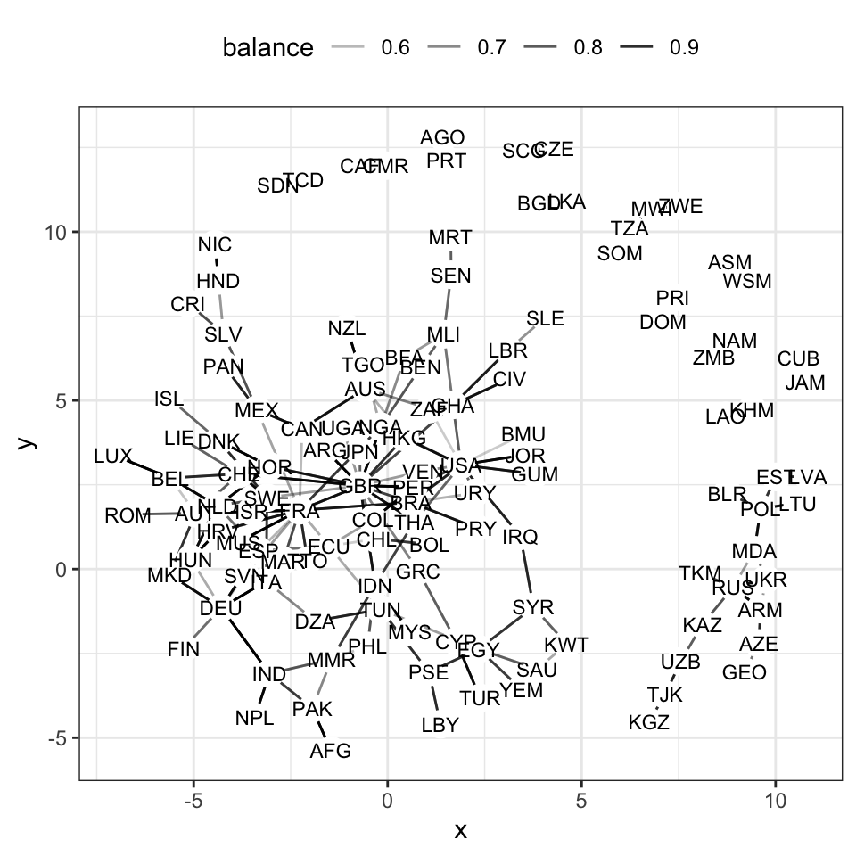
Even though the countries are not presented by geographic location, the network helps to illustrate the patterns of affinity between countries. Great Britain (GBR), the USA, and France (FRA) each are hubs having affinities with several countries. Egypt (EGY) is the center of an Arabic network connecting Saudi Arabia, Yemen, Kuwait, Palestine, Syria, and Tunisia. Another cluster centered on Russia (RUS) connects countries formed after the break-up of the Soviet Union.
14.4 Exercises
Problem 14.1: Here is a network
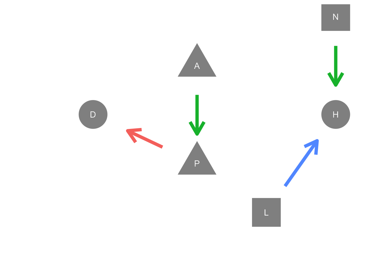
Which table gives the information needed to draw the edges in the graph?
| Table 1 | Table 2 | Table 3 | ||
|---|---|---|---|---|
| A -> P | A -> P | P -> A | ||
| H -> D | P -> D | P -> N | ||
| L -> H | L -> H | H -> L | ||
| A -> N | N -> H | N -> H |
Problem 14.2: For this network …
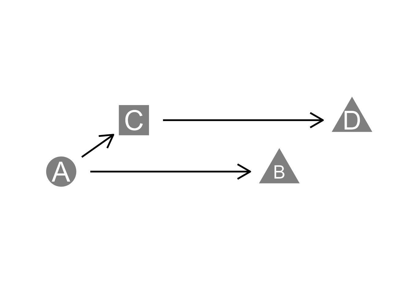
- What are the vertices?
- Which of these tables shows the edges correctly?
| Table 1 | Table 2 | Table 3 | ||
|---|---|---|---|---|
| A -> C | A -> C | A -> C -> D | ||
| B -> C | A -> B | C -> D | ||
| A -> B | C -> D |
- Explain what’s wrong with each of the other tables.
Problem 14.3: Consider this table of edges:
| from | to |
|---|---|
| China | Japan |
| USSR | Japan |
| Germany | USA |
| France | Germany |
| Italy | France |
| Germany | UK |
| Japan | UK |
| USA | Japan |
| USSR | Germany |
- How many distinct vertices are there?
- How many edges are there?