Chapter 11 Joining two data frames
The data verbs introduced so far — summarise(), mutate(), arrange(), and so on — always take as input a single data frame along with other arguments to specify the exact operation to be carried out. This chapter introduces data verbs that take two tables as input and produce a single table as output. Such operations enable you to combine information from different tables. With these two-table verbs, you can construct data-wrangling processes that combine many data frames. Arithmetic operations such as \(+\), \(-\), $ imes$, and \(\div\) combine two numbers, e.g. \(3+7\). Using such simple operations, you can construct more complicated ones that combine many numbers, e.g. \(3*(5/4 + 7)\). The two-table verbs can be used in analogous ways to combine information from multiple tables.
There are many situations where data from different sources have to be brought together to create a complete picture. For instance, the CountryData in Chapter 10 does not include even simple information about the geographic locations of the countries. If you want to plot the demographic data on a map, you will need to provide some geographic location data, as in CountryCentroids (from the dcData package).
Table 11.1: Two data frames, Demographics and CountryCentroids, with information about countries. In order to make a graphic with the demographic information shown on a map, a single glyph-ready table needs to be constructed by joining the information in both tables.
| country | pop | area |
|---|---|---|
| Afghanistan | 31822848 | 652230 |
| Akrotiri | 15700 | 123 |
| Albania | 3020209 | 28748 |
| Algeria | 38813722 | 2381741 |
| American Samoa | 54517 | 199 |
| … and so on for 256 rows altogether. |
| name | iso_a3 | long | lat |
|---|---|---|---|
| Afghanistan | AFG | 66.168500 | 33.78231 |
| Albania | ALB | 20.259880 | 41.14326 |
| Algeria | DZA | 2.828547 | 28.14225 |
| American Samoa | ASM | -170.723560 | -14.29717 |
| … and so on for 240 rows altogether. |
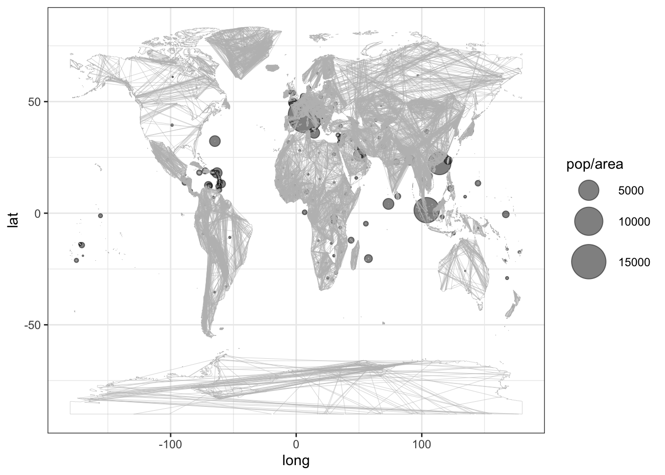
By combining the information in the two tables you can make a plot such as Figure 11.1 showing population density arranged geographically for each country.
Figure 11.1: Population density shown as dot area. Country borders are a graphics layer produced by mWorldMap().
Glyph-ready data for the scatter-plot component of Figure 11.1 has the form of Table 11.2. This is a combination of the tables from Demographics and CountryCentroids. But what kind of combination is it?
Table 11.2: Glyph-ready data for Figure 11.1.
| country | iso_a3 | long | lat | pop | area |
|---|---|---|---|---|---|
| Afghanistan | AFG | 66.168500 | 33.78231 | 31822848 | 652230 |
| Albania | ALB | 20.259880 | 41.14326 | 3020209 | 28748 |
| Algeria | DZA | 2.828547 | 28.14225 | 38813722 | 2381741 |
| American Samoa | ASM | -170.723560 | -14.29717 | 54517 | 199 |
| Andorra | AND | 1.534082 | 42.52563 | 85458 | 468 |
| … and so on for 191 rows altogether. |
Note first that Demographics and CountryCentroids have different numbers of rows, 256 and 240 respectively. Also note that the second row in Demographics is a different case entirely from the second row in CountryCentroids. So the glyph-ready data is not simply a cut-and-paste job of the long and lat variables of CountryCentroids as new variables conjoined to Demographics.
In combining Demographics and CountryCentroids to construct the glyph-ready data, a match is made between corresponding rows, even when they are in different positions in the two tables. For instance, row 7 in Demographics has been matched to row 4 in CountryCentroids. What these two rows have in common is that they both represent the data for Angola within their respective data frames.
To join Join: A data verb that finds matching rows in each of two data frames – referred to as the left and the right tables – and constructs an output that combines the data from the two tables accordingly. is a data verb that looks for information to match rows in one table to zero or more rows in a second table. Conventionally, the two tables are referred to as the left and the right table. The R/dplyr syntax is:
11.1 Variables for Matching
What does it mean for a case in the Left table to match a case in the Right table? A match is defined in terms of one or more variables that appear in both the Left and the Right tables. For each case in the Left table has values for the matching variable(s) that are identical to the values for the corresponding matching variable(s) in the Right table, a match between the Left case and the Right case is established.
Table 11.3 displays data on human migration between countries from dcData::MigrationFlows. Each case in MigrationFlows registers migration from an origin country to a destination country.
Table 11.3: The first several cases in the MigrationFlows data frame. (Not all variables are shown.) Each case is about migration from one country to another: the “origin” and “destination” countries. Country names are given using the three-letter ISO-A3 code. For instance, the migration to France (FRA) from Algeria (DZA) is conspicuously large.
| destcode | origincode | Y2000 |
|---|---|---|
| FRA | AFG | 923 |
| FRA | DZA | 425229 |
| FRA | AUS | 9168 |
| … and so on for 107,184 rows altogether. |
Suppose your interest in these data is to understand the forces that shape migration. Variables from dcData::CountryData, could be useful here. Table 11.4 selects a few health measures for each country: life expectancy, infant mortality, and fraction of the population considered underweight.
Table 11.4: CountryData: Health-related data from the CIA World Factbook data. Note that the country is identified by its common name.
| country | life | infant |
|---|---|---|
| Afghanistan | 50.49 | 117.23 |
| Akrotiri | NA | NA |
| Albania | 77.96 | 13.19 |
| Algeria | 76.39 | 21.76 |
| American Samoa | 74.91 | 8.92 |
| Andorra | 82.65 | 3.69 |
| … and so on for 256 rows altogether. |
Consolidating the health-related data to the migration data is done with a join. For instance, suppose you want to bring side-by-side the health data for the “origin” country and the migration data. To do this, you’ll have to match the origincode variable in MigrationFlows to the country variable in CountryData. It’s easy enough to do this for those countries whose code you can figure out, e.g. FRA for France, AFG for Afghanistan, etc. Common sense tells you to look up those codes you don’t already know, e.g. AUT for Austria and AUS for Australia.
Data-wrangling software will construct a match only when the information is in exactly the same form. So, while AUT is equivalent to Austria, you need to demonstrate this equivalence. In other words, you’ll need to find or construct a data frame that contains the translation from country code to country name. This sometimes requires creativity; it certainly requires a knowledge of what data are available. For instance, the dcData::CountryCentroids data frame (Table 11.5) lists both the country and the country code:
Table 11.5: Two variables selected from CountryCentroids.
| name | iso_a3 |
|---|---|
| Afghanistan | AFG |
| Aland | ALA |
| Albania | ALB |
| Algeria | DZA |
| … and so on for 241 rows altogether. |
To translate the country variable in CountryData to the iso_a3 code, join CountryCentroids to CountryData, producing 11.6.
InfantMortality <-
CountryCentroids %>%
select(name, iso_a3) %>%
left_join(CountryData %>% select(country, infant),
by = c("name" = "country")) Table 11.6: InfantMortality table produced by joining CountryCentroids to CountryData.
| name | iso_a3 | infant |
|---|---|---|
| Afghanistan | AFG | 117.23 |
| Aland | ALA | NA |
| Albania | ALB | 13.19 |
| Algeria | DZA | 21.76 |
| American Samoa | ASM | 8.92 |
| Andorra | AND | 3.69 |
| … and so on for 241 rows altogether. |
Note that the by argument to left_join() specifies that the case matching is to be accomplished by comparing the name variable in the Left table to the country variable in the Right table. Now you are in a position to join the infant mortality data to the migration data. The variables for matching will be iso_a3 in InfantMortality and destcode in MigrationFlows:
| sex | destcode | origincode | Y2000 | name | infant |
|---|---|---|---|---|---|
| Male | FRA | AFG | 923 | France | 3.31 |
| Male | FRA | DZA | 425229 | France | 3.31 |
| Male | FRA | AUS | 9168 | France | 3.31 |
| Male | FRA | AUT | 7764 | France | 3.31 |
| Male | FRA | AZE | 118 | France | 3.31 |
| Male | FRA | BLR | 245 | France | 3.31 |
| … and so on for 107,184 rows altogether. |
Often, the tables you are joining have the same name for corresponding variables. A natural join Natural Join: The selection of variables that match the cases in one table to another based simply on variables with the same name that appear in both tables. defines the matching cases by all the same-named pairs of variables. In other situations, the corresponding variables may have different names, or you may not want to join based on all the same-named pairs. In these situations, you can explicity identify the corresponding variables with the by argument.
Or, you could bring in infant mortality for the origin country:
| sex | destcode | origincode | Y2000 | Y1990 | Y1980 | Y1970 | Y1960 | name | infant |
|---|---|---|---|---|---|---|---|---|---|
| Male | FRA | AFG | 923 | 91 | 55 | 29 | 1471 | Afghanistan | 117.23 |
| Male | FRA | DZA | 425229 | 861691 | 794288 | 723746 | 521679 | Algeria | 21.76 |
| Male | FRA | AUS | 9168 | 903 | 1483 | 1906 | 14614 | Australia | 4.43 |
| Male | FRA | AUT | 7764 | 2761 | 4686 | 4861 | 12375 | Austria | 4.16 |
| Male | FRA | AZE | 118 | 12 | 20 | 4 | 188 | Azerbaijan | 26.67 |
| Male | FRA | BLR | 245 | 88 | 26 | 0 | 390 | Belarus | 3.64 |
| … and so on for 107,184 rows altogether. |
11.2 Different Types of Join
You’ve seen the role of matching variables in a join operation. When there is a match between a case in the Left table and a case in the Right table, the remaining variables from the Right table are concatenated onto the case from the Left table.
Some questions remain:
- What happens when a case in the Right table has no matches in the Left?
- What happens when a case in the Left table has no matches in the Right?
- What happens when there are multiple cases in the Left that match a case in the Right?
There are different answers that are appropriate in different situations. For that reason, there are a variety of join operators that work in different ways. A few of the more commonly encountered join operators include:
left_join()— the output has all the cases from the Left, even if there is no match in the right.inner_join()— the output has only the cases from the Left with a match in the Right.full_join()— the output will have all the cases from both the Left and the Right.
All of these join operators behave the same when there are multiple matches in the Right table for a case in the Left table: Each of these multiple matches will produce a case in the output.
11.3 Common Uses for Joins
Mutating
Mutating means to add new variables to a data frame. The mutate() data verb lets you add new variables constructed by transformation operations on existing variables. The join verbs can do something similar: constructing new variables by pulling them out of a different data frame.
Translating
One common sort of mutation deserves special attention. Often, you will need to translate levels in one variable into a different set of levels. You’ve already seen this in the MigrationFlows and CountryData task; Migration data had countries listed in ISO-code form, whereas CountryData has countries listed by name. The translation from one form to another happened to be described by the CountriesCentroid data.
Filtering
You can use the filter() function to extract those cases that meet a given criterion. Sometimes you may have a list of the cases you want. inner_join() lets you choose the cases you want in that list. For example, Table 11.7 lists the G8 countries. To extract the G8 cases from another table, use an inner join between that table and G8 country table as illustrated in Table 11.8.
Table 11.7: The G8 countries.
| country |
|---|
| Canada |
| France |
| Germany |
| Italy |
| Japan |
| Russia |
| United Kingdom |
| United States |
Table 11.8: An inner join of CountryData with G8 extracts just the G8 cases.
| country | GDP | pop |
|---|---|---|
| Canada | 1.518e+12 | 34834841 |
| France | 2.276e+12 | 66259012 |
| Germany | 3.227e+12 | 80996685 |
| Italy | 1.805e+12 | 61680122 |
| Japan | 4.729e+12 | 127103388 |
| Russia | 2.553e+12 | 142470272 |
| … and so on for 8 rows altogether. |
11.4 Exercises
Problem 11.1: Most data verbs, when used with the chaining syntax %>%, have arguments that consist only of reduction and transformation functions, constants, and variables. For instance:
In contrast, the join family of data verbs — inner_join(), left_join(), etc. — always have a data table as one of the arguments inside the parentheses. Explain why.
Problem 11.2: Consider these two tables containing demographic and geographic information about countries.
Table 11.9: Demographics
| country | pop | area |
|---|---|---|
| Afghanistan | 31822848 | 652230 |
| Akrotiri | 15700 | 123 |
| Albania | 3020209 | 28748 |
| Algeria | 38813722 | 2381741 |
| American Samoa | 54517 | 199 |
| Andorra | 85458 | 468 |
| … and so on for 256 rows altogether. |
Table 11.10: CountryCentroids
| name | iso_a3 | long | lat |
|---|---|---|---|
| Afghanistan | AFG | 66.168500 | 33.78231 |
| Aland | ALA | 19.967041 | 60.19722 |
| Albania | ALB | 20.259880 | 41.14326 |
| Algeria | DZA | 2.828547 | 28.14225 |
| American Samoa | ASM | -170.723560 | -14.29717 |
| Andorra | AND | 1.534082 | 42.52563 |
| … and so on for 241 rows altogether. |
Explain why the information in the two tables cannot be successfully combined by laying the two tables side by side into a single table, that is, by simply copying the long and lat variables from one table and pasting them alongside the country, pop and area variables in the other table.
Problem 11.3: Use the ZipGeography and ZipDemography data tables (from dcData) to create these graphics.
- Make a bar chart showing, for each state, the count of the population that is under 5 years old, between 5 and 18 years old, between 18 and 65 years old, and over 65.
- Make another bar chart showing the proportion of the state population that is in each of the age categories.
- Call a ZIP code “crowded” when the population is over 50,000. Make a scatter plot showing the geographic location of the crowded ZIPs.
- Make a choropleth map of the US showing, for each state, one of the following (your choice). Hint: you’ll have to sum over all the ZIP codes in a state before you can meaningfully find the fraction.
- the fraction of housing units (
Totalhousingunits) that are vacant (Vacanthousingunits).
- the fraction of the population that is over 65 years old.
- the fraction of the population with a bachelor’s degree (
Bachelorsdegreeorhigher).
- the fraction of housing units (
- Pick out the 10,000 zip codes with the highest population. Make a scatter plot of the latitude versus longitude. (Hints:
arrange()andhead().) Use color to represent the fraction of the population that is over 65.
- How many zip codes have a
WaterAreathat is more than 50% of theLandArea? Make a scatter plot showing the geographical location of these, with color indicating the population.
Problem 11.4: Make a scatterplot map of the locations of the Medicare providers. (Hint: the ZIP code provides this information. You can translate it into latitude and longitude with ZipGeography.) Overlay this on a choropleth map giving the population of each state.
Problem 11.5: Using the ZipGeography data table (from dcData), answer the following questions. In addition to the answer itself, show the statement that you used and the data table created by your statement that contains the answer.
- How many different counties are there?
- Which city names are used in the most states?
- Identify cities that include more than 5% of their state population; which of those city names are used in the most states?
- Does any state have more than one time zone?
- Does any city have more than one time zone?
- Does any county have more than one time zone?
Problem 11.6: Migration and Mortality
One possible driver of migration is that it tends to be from countries with high infant mortality to those with low mortality.
Here are two data tables that might be used answer a research question: does migration tend to be from high infant-mortality countries to low infant-mortality countries? To answer this question, a glyph-ready data table like this would be useful.
| sex | countryA | countryB | toAfromB | toBfromA | infantA | infantB |
|---|---|---|---|---|---|---|
| Male | BRA | JPN | 92718 | 141 | 19.21 | 2.13 |
| Male | USA | JPN | 47140 | 6520 | 6.17 | 2.13 |
| Female | BRA | JPN | 73942 | 106 | 19.21 | 2.13 |
| Female | USA | JPN | 67841 | 5970 | 6.17 | 2.13 |
| Male | CAN | NOR | 13678 | 371 | 4.71 | 2.48 |
| Male | SWE | NOR | 13877 | 7997 | 2.60 | 2.48 |
| Male | USA | NOR | 84071 | 3897 | 6.17 | 2.48 |
| Female | SWE | NOR | 22847 | 9359 | 2.60 | 2.48 |
| Female | USA | NOR | 75232 | 4652 | 6.17 | 2.48 |
| Male | CAN | SWE | 11985 | 328 | 4.71 | 2.60 |
| Male | USA | SWE | 116413 | 4854 | 6.17 | 2.60 |
| Female | DNK | SWE | 12189 | 15746 | 4.10 | 2.60 |
| … and so on for 628 rows altogether. |
This glyph-ready table could be constructed from the MigrationFlows data table and the HealthIndicators data table.
Table 11.11: MigrationFlows
| sex | destcode | origincode | Y2000 |
|---|---|---|---|
| Male | FRA | CAN | 9859 |
| Male | FRA | MEX | 1214 |
| Male | CAN | FRA | 17983 |
| Male | CAN | MEX | 2863 |
| Male | MEX | CAN | 2880 |
| Male | MEX | FRA | 2231 |
| … and so on for 12 rows altogether. |
Table 11.12: HealthIndicators
| iso_a3 | infant |
|---|---|
| CAN | 4.71 |
| FRA | 3.31 |
| MEX | 12.58 |
Your task is to figure out the data wrangling steps to get from the two input tables to the glyph-ready table.
To start, fill in this blank table by hand with the right entries from the input tables. Assume that countryB in the glyph-ready data corresponds to origincode in MigrationFlows. This will help you be better able to appreciate the individual data wrangling steps.
| sex | countryA | countryB | toAfromB | toBfromA | infantA | infantB |
|---|---|---|---|---|---|---|
| Female | CAN | FRA | ||||
| Female | FRA | MEX | ||||
| Male | CAN | MEX |
Now, answer these questions.
- How will you create a data table from
MigrationFlowsthat renamesorigincode,destcode, andY2000tocountryB,countryAandtoAfromB? - While
toAfromBcomes directly fromMigrationFlows, the reverse flow,toBfromA, needs to be brought in via a join. What pairs of variables are being matched for the join?
- Both
infantAandinfantBcome fromHealthIndicators. What variables are being matched forinfantA? - What variables are being matched for
InfantB?