Chapter 3 Basic R Commands
Almost everyone who writes computer commands starts by copying and modifying existing commands. To do this, you need to be able to read command expressions. Once you can read, you will know enough to identify the patterns you need for any given task and consider what needs to be modified to suit your particular purpose.
As you read this chapter, you will likely get an inkling of what the commands used in examples are intended to do, but that’s not what’s important now. Instead, focus on
- Distinguishing between functions and arguments.
- Distinguishing between data tables and the variables that are contained in them.
- Recognizing when a function is being used.
- Identifying the arguments to a function.
- Observing how assignment allows values to be stored and referred to by name.
- Discerning when the output of one function becomes the input to another.
You are not expected at this point to be able to write R expressions. You’ll have plenty of opportunity to do that once you’ve learned to read and recognize the several different patterns used in R data wrangling and visualization commands.
3.1 Language Patterns and Syntax
In a human language like English or Chinese, syntax is the arrangement of words and phrases to create well-formed sentences. For example, “Four horses pulled the king’s carriage,” combines noun phrases (“Four horses”, “the king’s carriage”) with a verb.
Consider this pair of English language sentence patterns, a statement and a question:
- I did go to school .
- Did I go to school ?
The content of each of the boxes can be replaced by an equivalent object.
- I can be replaced with “you”, “we”, “he”, “Janice”, “the President”, and so on.
- go to can be replaced with “stay in”, “attend”, “drive to”, “see”, …
- school can be replaced with “the lake”, “the movie”, “Fred’s parents’ house”, …
Such replacements produce sentences like these:
- Did we stay in Fred’s parents’ house?
- Janice did drive to the lake.
- Did the President see the movie?
- Did he attend school?
Each sentence expresses something different, but they all follow the same patterns.
R has a few patterns that suffice for many data wrangling and visualization tasks. Consider these patterns:
object_name
<-function_name(arguments)
This is called function application. The output of the function will be stored under the name to the left of<-.object_name
<-Data_frame%>%function_name(arguments)
This is called chaining syntax.object_name
<-Data_frame%>%
function_name(arguments)%>%function_name(arguments)
This is an extended form of chaining syntax. Such chains can be extended indefinitely.
3.2 Five kinds of objects
There are five kinds of objects that you will be working with extensively.
- Data tables
- Functions
- Arguments
- Variables
- Constants
Just as it helps in English to know what’s a noun and what’s a verb, etc., by identifying each kind of object in an expression you’ll have an easier time understanding what the expression does.
1. Data tables contain tidy data. A data table comprises one or more variables. Data tables appear at the start of a chain, just before the first %>%.
2. Functions are the objects that transform an input into an output. They are easy to spot because the function name will always be followed immediately by an open parenthesis. In between this open parenthesis and the corresponding closing parenthesis typically one or more arguments are specified. There are a few functions that have a different syntax. For example, simple mathematical functions are placed between two arguments, e.g., 3 + 2 or 7 * 8. This is called infix notation and is meant to mimic traditional arithmetic notation. Some other infix functions you’ll encounter are %in%, ==, >=, and so on.
3. Arguments specify inputs and other details that dictate what the function is to do. They appear between the parentheses that follow a function name. One important exception: data tables are typically presented as an input to a function using the chaining notation %>%.
Many functions take named arguments where the name of the argument is followed by a = sign and then the value of that argument. For instance, by = x gives x as the value of the argument named by. In other cases, it is not necessary to specify any arguments at all between the opening and closing parentheses corresponding to a function. Since functions have different purposes, they do not necessarily require the same inputs so arguments do not generally transcend functions. For example, a named argument that is appropriate for one function may not be appropriate for another function or may have a different meaning when used in different functions. Reviewing the R help for a function is a good way to learn about the names, types, and purposes of various arguments available to that function.
4. Variables are the columns in a data table. In this book, they will always be in function arguments, that is, between parentheses.
5. Constants are single values, most commonly a number or a character string. Character strings will always be in quotation marks, "like this." Numerals are the written form of numbers, for instance -42, 1984, 3.14159. Sometimes you’ll see numerals written in scientific notation, e.g. 6.0221413e+23 or 6.62606957e-34.
To help distinguish data frames from the variables in them, these notes will use a simple naming convention.
- The names of data tables will start with a CAPITAL letter. For instance:
WorldCities,NCI60,BabyNames, and so on. - The names of variables within data tables will start with a lower-case letter. For instance:
latitude,country,population,date,sex,count,countryRegion,population_density.
To be clear, these conventions are style choices, not rules enforced by the R language. As you create your own data tables and variables, it is up to you to follow the convention. Even in this book you will encounter data or variables that fail to follow this convention, particularly in situations that rely on resources developed by other people or institutions who don’t follow these conventions.
Conforming to a consistent programming style makes R code easier for people to read. Just as there are complete, yet distinct, syle guides for consistent writing standards (e.g., MLA, APA, Chicago) relatively complete style guides for R programming exist as well. To be clear, these conventions are style choices, not rules enforced by the R language. As you create your own data tables and variables, it is up to you to follow the convention. Even in this book you will encounter data or variables that fail to follow this convention, particularly in situations that rely on resources developed by other people or institutions who don’t follow these conventions. One such style guide accompanies this book as an appendix.
Example: Classifying objects in an expression
Consider this command:
The statement involves a data table (hint: starts with a capital letter, not followed by a opening parenthesis), three functions (hint: look for the names followed by an opening parenthesis), a named argument total (hint: inside the parentheses and followed by a single equal sign). The string "Arjun" is a constant. The remaining names — name and count — are variables. (Hint: they are involved in the arguments to functions).
The filter() function is being given the argument name == "Arjun". This can be confusing. Although == somewhat resembles =, the single = is always just punctuation in a named argument. The double == is a function — one of those few infix functions that don’t involve parentheses.
By the way, the overall effect of the command is to calculate the total number of individuals named Arjun represented in the BabyNames data. The result of the calculation is 5,578. Try it yourself!
Note to experienced programmers. You may be wondering where common programming constructs like looping and conditional flow, indexing, lists, and function definition fit in with this book. This book uses a couple of domain-specific, sub-languages, particularly dplyr and ggplot2. A “sub-language” is a part of a computer language that can be used almost like a language of it’s own. The functions in dplyr and ggplot2 already contain within them those programming constructs, so there is no need to use them explicitly. This is analogous to driving a car. The sub-language is the use of the steering wheel, brake, and accelerator. You can use these to accomplish your task without having to know about how the engine or suspension work.
3.3 Example Expressions
These are expressions that you will use frequently, each written in the chaining style. To remind you, BabyNames is a data table.
Expressions that give a quick glance at a data table
These functions are generally used interactively, in the R console, to help you when constructing expressions for data wrangling or visualization.
## [1] 1792091## [1] "name" "sex" "count" "year"| name | sex | count | year |
|---|---|---|---|
| Mary | F | 7065 | 1880 |
| Anna | F | 2604 | 1880 |
| Emma | F | 2003 | 1880 |
## 'data.frame':	1792091 obs. of  4 variables:
##  $ name : chr  "Mary" "Anna" "Emma" "Elizabeth" ...
##  $ sex  : chr  "F" "F" "F" "F" ...
##  $ count: int  7065 2604 2003 1939 1746 1578 1472 1414 1320 1288 ...
## $ year : int 1880 1880 1880 1880 1880 1880 1880 1880 1880 1880 ...## Rows: 1,792,091
## Columns: 4
## $ name <chr> "Mary", "Anna", "Emma", "Elizabeth", "Minnie", "Margaret", "Ida…
## $ sex <chr> "F", "F", "F", "F", "F", "F", "F", "F", "F", "F", "F", "F", "F"…
## $ count <int> 7065, 2604, 2003, 1939, 1746, 1578, 1472, 1414, 1320, 1288, 125…
## $ year <int> 1880, 1880, 1880, 1880, 1880, 1880, 1880, 1880, 1880, 1880, 188…Modifying a data table
Sometimes, you will want to modify a data table and store the result under the original name. To illustrate:
Because assignment is being used to capture the value being created by filter(), it might look like nothing is being done. But, behind the scenes, BabyNames has changed.
## [1] 27890| name | sex | count | year |
|---|---|---|---|
| Emily | F | 26177 | 1998 |
| Hannah | F | 21368 | 1998 |
| Samantha | F | 20191 | 1998 |
| Ashley | F | 19868 | 1998 |
Of course, it’s not necessarily to use the original name to store the result of the modification. You can use any name that you think appropriate.
Named arguments and functions in arguments
The previous example – BabyNames %>% head(4) – involved an argument to a function; head() is given the number 4 to specify how many cases to show. Sometimes the arguments will be the name of a variable or a function applied to a variable. Here’s an example:
| sex | total |
|---|---|
| F | 1765766 |
| M | 1910081 |
Taking apart the above expression, you can see three functions: group_by(), summarise() and sum().The group_by() and summarise() functions will be described in Chapter 4. They are called data verbs because they each take a data table as an input and produce a data table as output. The name of functions is always followed by an open parenthesis. Inside those parentheses are the arguments. The argument to group_by() is sex, a variable. How do you know? It’s evidently not a data table — it’s not capitalized. It’s neither a character string nor a numerical constant. And it’s not a function — sex isn’t followed by an opening parenthesis. By the process of elimination, this suggests that sex is a variable. The argument to summarise() is the expression total = sum(count).
The argument to summarise() is in named-argument form. Note that sum() is a function. You can tell this from the expression: sum is followed immediately by an open parenthesis.
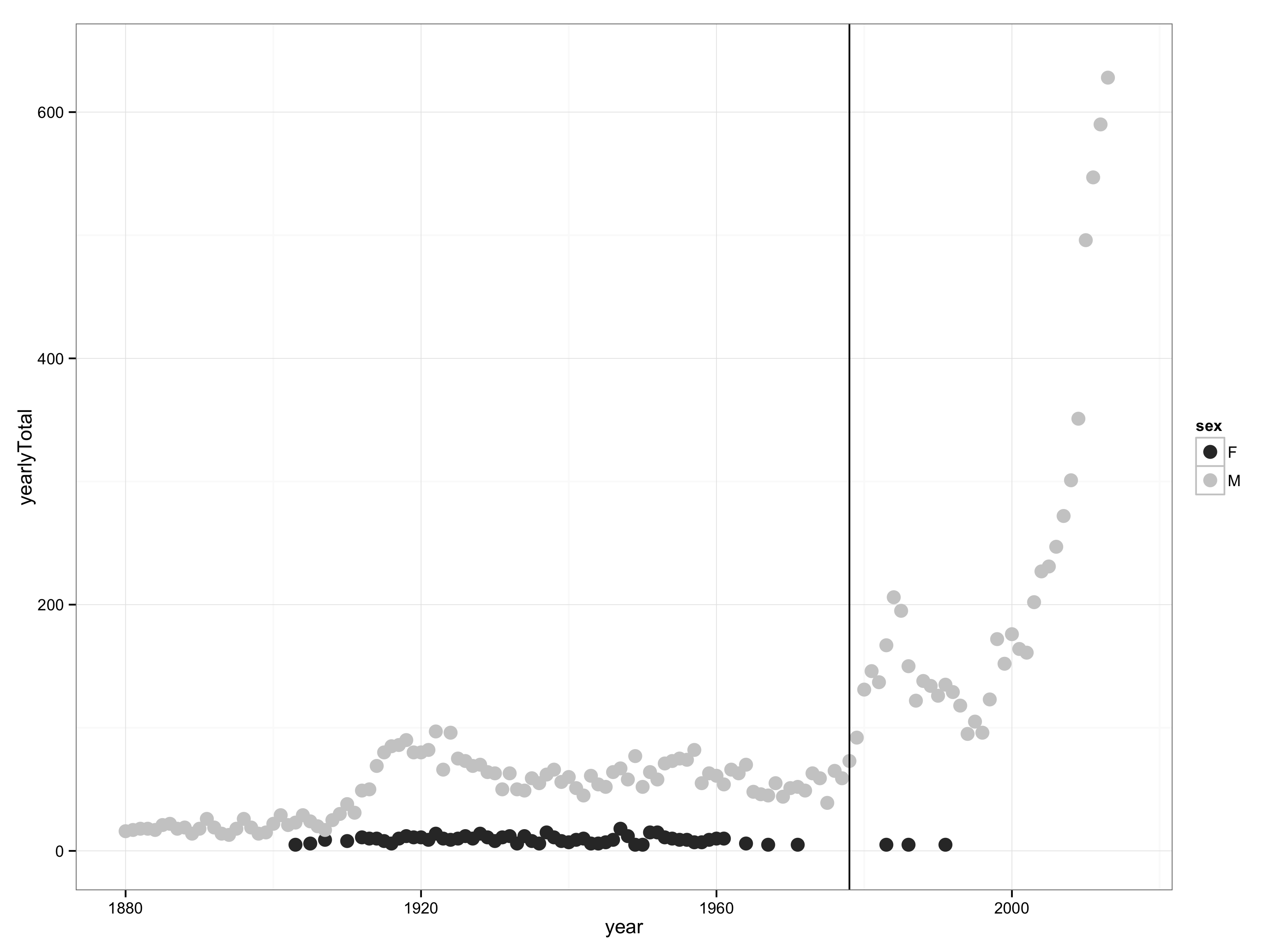
Figure 3.1: The number of babies born each year given the name “Prince”.
3.4 Example: A genuine data wrangling computation
What do realistic data wrangling and graphics expressions look like? Figure 3.1 depicts the popularity of the name “Prince” as it varies over the years. (Don’t worry for now about what the various functions are doing. You will get to that later.)
Princes <-
  BabyNames %>%
  filter(name == "Prince") %>%
  group_by(year, sex) %>%
  summarise(yearlyTotal = sum(count))

# Now graph it!
Princes %>%
  ggplot(aes(x = year, y = yearlyTotal)) +
  geom_point(aes(color = sex)) +
  geom_vline(xintercept = 1978) +
  ylim(0,640) + xlim(1880,2015)
Judging from Figure 3.1, the name “Prince” has been increasing in popularity over the last 40 years. One possible explanation is the popularity of the musician, Prince. The vertical line in the graph marks the year that Prince’s first album was released: 1978.
3.5 Constant objects
Sometimes you will use assignment to store a constant. Reminder: The two kinds of constants we will use are quoted character strings and numerals. For instance:
Naming constants in this way can help to make your data wrangling expressions more readable. For instance, by using age_cutoff in your expressions, you make it easily to update your expressions if you decide to change the age cutoff; just change the 21 to whatever the new value is to be.
3.6 Chaining syntax
If you have experience with R, you may never have seen the chaining operator %>% before this book.
Chapter 2 showed several different examples of function application, function_name ( arguments ), for instance sqrt(2) and help(CPS85, package="mosaic")
Chaining syntax is merely another form of function application. The following two patterns accomplish exactly the same thing:
Chaining pattern: Data_frame %>% function_name ( arguments )
Non-chaining pattern: function_name ( Data_Table , arguments )
In chaining syntax, the value on the left side of %>% becomes the first argument to the function on the right side. Note also that %>% is never at the start of a line — it should be placed at the end of any line which is to be followed by another step in a command sequence.
The chaining syntax is a help to the human reading and writing computer commands. Chaining makes more prominent the functions at each step. This is particularly helpful when there are many steps in a data wrangling or visualization task. To illustrate, here’s a command sequence used previously in this chapter:
Princes <-
  BabyNames %>%
  filter(name == "Prince") %>%
  group_by(year, sex) %>%
  summarise(yearlyTotal = sum(count))
This expression can also be written in a non-chaining syntax, for instance:
Princes <-
  summarise(
    group_by(
      filter(BabyNames, name == "Prince"),
      year, sex),
    yearlyTotal = sum(count))
The chaining syntax takes advantage of the nature of data verbs. Each step in a data wrangling sequence takes a data table along with some other arguments as input and produces a data table as output. The chaining sequence brings the other arguments much closer to the data verb itself, so that you can see at a glance which arguments belong to which data verbs. For those just beginning to read the chaining syntax, the %>% operator (sometimes called a “pipe”) to approximately translate to mean “and then” within the context of a chain of R commands. For example, we started with the BabyNames data, and then filter it based on name, and then group by year and sex, and then summarize the result.
3.7 Exercises
Problem 3.1: For each of the following, make up an R expression that uses an object named fireplace. The expression should have enough context to be able to identify the name as belonging to
- a data table
- a function
- the name of a named argument
- a variable
Problem 3.2: Explain why the following sentence is illegitimate:
Result <- %>% filter(BabyNames, name=="Prince")
Problem 3.3: Consider these R expressions. (You don’t have to know what the various functions do to solve this problem.)
# prepare the data
Princes <-
  BabyNames %>%
  filter(name == "Prince") %>%
  group_by(year, sex) %>%
  summarise(yearlyTotal = sum(count))

# now graph it!
Princes %>%
  ggplot(aes(x = year, y = yearlyTotal)) +
  geom_point(aes(color = sex)) +
  geom_vline(xintercept = 1978)
There are several kinds of named objects in the above expressions.
- function name
- data table name
- variable name
- name of a named argument
Using the naming convention and position rules, identify what kind of object each of the following name is used for. That is, assign one of the types (a) through (d) to each name.
1) BabyNames |
2) filter |
3) name |
4) == |
5) group_by |
6) year |
7) sex |
8) summarise |
9) sum |
10) count |
11) ggplot |
12) aes |
13) x |
14) y |
15) geom_point |
16) color |
17) geom_vline |
18) xintercept |
Challenge: Notice that YearlyTotal seems to represent more than one kind of object in the R expressions shown previously. Here, assign one of the types (a) through (d) to each excerpt where YearlyTotal was used:
19) summarise(yearlyTotal = sum(count)) |
20) ggplot(aes(x = year, y = yearlyTotal)) + |
Problem 3.4: There are several small, example data tables in the ggplot2 package. Look at the msleep data table by using the View() function with the name of the object as an argument. You may also need to review the documentation with help().
- What is the meaning of the
brainwtvariable? - How many cases are there?
- What is the real-world meaning of a case?
- What are the levels of the
vorevariable?
Problem 3.5: The data verb functions all take a data frame as their first argument and return a data frame as their output. The chaining syntax lets the output of one function become the input to the following function, so you don’t have to repeat the name of the data frame. An alternative syntax is to assign the output of one function to a named object, then use the object as the first argument to the next function in the computation.
Each of these statements, but one, will accomplish the same calculation. Identify the statement that does NOT match the others.
BabyNames %>%
  group_by( year, sex ) %>%
  summarise( totalBirths=sum(count))
group_by( BabyNames, year, sex) %>%
summarise( totalBirths=sum(count) )group_by( BabyNames, year, sex ) %>%
summarise( totalBirths=mean(count) )Tmp <- group_by(BabyNames, year, sex)
summarise( Tmp, totalBirths=sum(count) )Problem 3.6: The date() function returns an indication of the current time and date.
- What arguments does
date()take? Usehelp()to find out. - What kind of object is the result from
date().
Problem 3.7: Newcomers often get confused about the difference between a quoted character string and an object name. You’re going to explore the difference using the View() function. View() lets you see the contents of objects.
- Look briefly at the documentation, via the
help()function, for the data tablemsleep(in theggplot2package). - Look at the data table itself:
View(msleep) - Now do the same thing, but using the quoted character string
"msleep"rather than the name of the object. That is,View("msleep").
In your own words, briefly explain the difference between msleep and "msleep".