Chapter 2 Computing with R
Data frames are often large, so it is not possible to undertake paper-and-pencil operations on them. The BabyNames data frame introduced previously provides a case in point. BabyNames has 1,790,091 rows, far too many to carry out by hand even a simple sum or count. Data science relies on computers.
The human role in the process is managerial, to decide what forms of analysis are called for by the purpose at hand and to instruct the computer to carry out the operations needed. The process of instructing a computer is called computer programming.1 The process of writing instructions for a computer. Sometimes the unfortunate word “coding” is used. The point of programming is to make instructions clear, not to obscure them with code. Programming is done using a language that is accessible both to humans and the computer; the human writes the instructions and the computer carries them out. These notes use a computer language called R.
This chapter introduces concepts that underlie the use of R. The emphasis here will be on the kinds of things that R commands involve. Only a few R commands will be covered, but these will illustrate the most important patterns in writing with R. Chapter 3 will start to introduce the commands themselves that are used for working with data.
2.1 R and RStudio
The R language includes many useful operations for working with data, drawing graphics, and writing documents, among other things.
RStudio is a computer application that gives ready access to the resources of R. RStudio provides an interface for organizing for organizing your work and interacting with R. There are other ways to work with R, but for good reason RStudio has become the most popular. RStudio offers facilities both for newbies and for professionals; it’s good for everybody.
RStudio comes in two versions:
- A desktop that runs on the user’s own computer.
- A server that runs on a computer in the cloud and is accessed by a web browser.
You can install R and the desktop version of RStudio on all the most common operating systems: OS-X, Windows, Linux. There are now many text and video guides to installation. See marin-stats-lectures for an example.
If you are to use the server version of RStudio, someone has set up a server for you and provided a login ID. You access the server through an ordinary web browser — Chrome, Firefox, Safari, etc. — that may be running on a laptop, a tablet, or even a smartphone.
The two RStudio versions, desktop or server, are almost identical from a user’s point of view. The desktop version is often faster but can only be used on one computer; the server version requires almost no set-up and is available from any computer browser but may slow down when there are many simultaneous users, as might happen in a classroom.
2.2 Components of the RStudio application
Just as a window in a house has several individual panes of glass, so the RStudio application appears in an graphical interface window divided up into several panes. All panes can be viewed at the same time. Each of the panes can contain several tabs.
Figure 2.1: The RStudio window is divided into four panes. Each pane can contain multiple tabs.
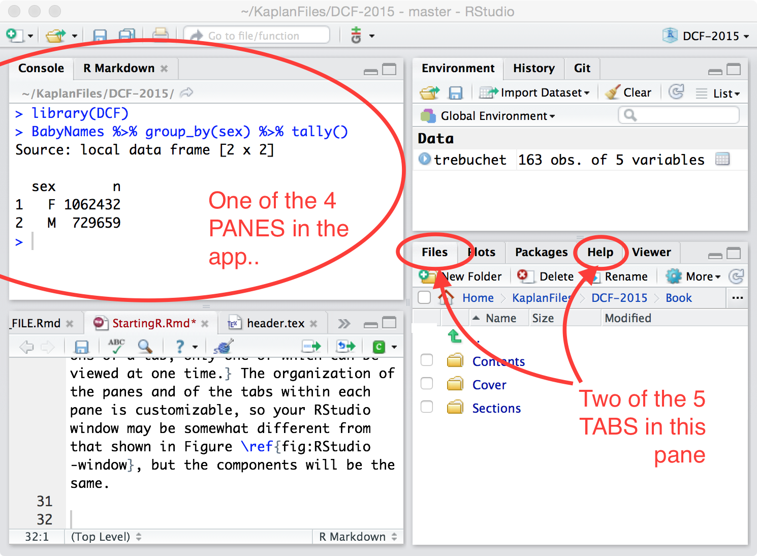
The organization of the panes and of the tabs within each pane is customizable, so your RStudio window may be somewhat different from that shown in Figure 2.1.
You will often be using the Console tab and tabs for editing documents. Each document-editing tab has the name of the document it contains. In Figure 2.1, three such editing tabs are shown, one of which is labeled StartingR. Other important tabs: Packages for installing new R software and Help for displaying documentation.
2.3 Commands and the Console
This is a good time to start up your version of RStudio. Once RStudio is running:
- Enter R-language commands into the console. Find the console tab in your RStudio app and the prompt,
>. - Move the cursor to the console tab so that anything you type shows up there. Type the simple command shown in Figures 2.2, 2.3, and 2.4.
- After you press enter, \(\hookleftarrow\), R will execute your command and print out a response.
Figure 2.2: The console tab showing the command prompt > .
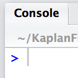
Figure 2.3: The console tab showing a command composed but not yet entered.
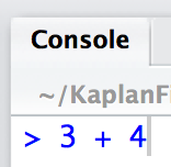
Figure 2.4: The console tab after entering the command.
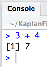
Notice that after the response, there is another prompt. You’re ready to go again.
Practice. Enter each of the following arithmetic commands at the command prompt, one at a time. Confirm that the response is the right arithmetic answer.
16 * 9
sqrt(2)
20 / 5
18.5 - 7.21
2.4 Sessions
Your work in R occurs in sessions. A session is a kind of ongoing dialog with the R system.
A new session is begun every time you start RStudio. The session is terminated only when you close or quit the RStudio program. If you are using RStudio server (via your browser), the R session will be maintained for days or weeks or months, and will be retained even when you login to the server from a different computer.
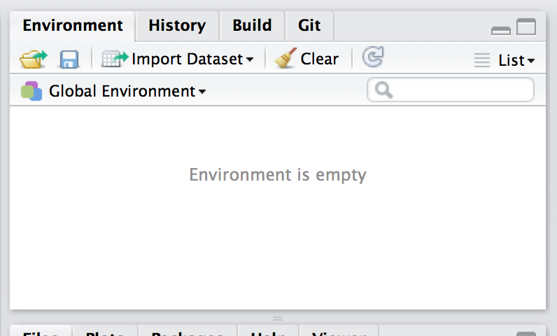
When a session is first started, it is in an empty environment. RStudio displays this in the Environment tab. (Figure 2.5)
Figure 2.5: The “Environment” tab in RStudio lists the objects in the "session environment." At the start of a session, the environment is empty.
2.5 Packages
Many people work to provide and maintain new software and new capabilities for R. Such additions are called packages. Among the packages you will be using, the dcData package contains data for the examples in this book, and the tidyverse package provides access to lots of wrangling and visualization tools to be introduced. In order to make resources in dcData accessible, you have to load. The command is:
Usually you will give this command at the start of a session or at the top of a document.
Did something go wrong?
In response to the above command, you might get a response from R like this:
Error in library(dcData) : there is no package called ‘dcData’If this happens, it means only that your R account is not up to date with the dcData package and you will have to install the package. To do so, use these two commands in sequence. (Copy the commands verbatim into your R console. The installation may take some minutes depending on the speed of your Internet connection)
Then try again: Many users will find it useful to also install the more complete DataComputing package – devtools::install_github("DataComputing/DataComputing") – which augments the data sets available in dcData with additional functionality used in this book.
R has lots (and lots) of packages. While dcData is hosted by a remote server called (GitHub)[http://github.com/], many others are hosted and installed from the Comprehensive R Archive Network (CRAN). The line install.packages("devtools") shown previously actually installed a package called devtools from CRAN. Technically, tidyverse is just a wrapper for a “collection of R packages designed for data science” to be installed and loaded all at once. You can learn more about the Tidyverse at https://www.tidyverse.org/. The tidyverse package can also be installed from CRAN.
2.6 Data
The data you work with will be organized into data frames. Data frames are generally stored in files or database systems or even web pages. To use a data table in R, you need to read the data into your R session. There are many ways to do this. The simplest, and the one we will use in this introduction, is via the data() function.
You can list the data in a package with this command:
The command shows a table like the following in an editing tab:
| Item | Title |
|---|---|
| BabyNames | Names of children as recorded by the US Social Security Administration. |
| CountryGroups | Membership in Country Groups |
| HappinessIndex | World Happiness Report Data |
| MedicareCharges | Charges to and Payments from Medicare |
| … and so on for 20 rows altogether. |
To read a data table into R from the dcData package, use the data() function with the name of the data table and the name of the package, as in:\index{data!read into R’)`
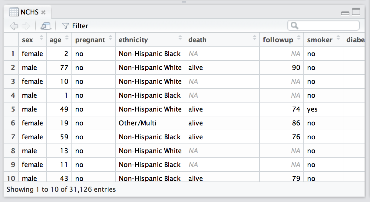
To take a peak at the data that has already been read into an ongoing session, use View(). This will display the object in a new tab as in Figure 2.6.
Figure 2.6: The tab opened by RStudio in response to View(NCHS).
Another way to get information about the data is to click on the expand icon, ![]() next to the NCHS listing in the environment tab.
next to the NCHS listing in the environment tab.
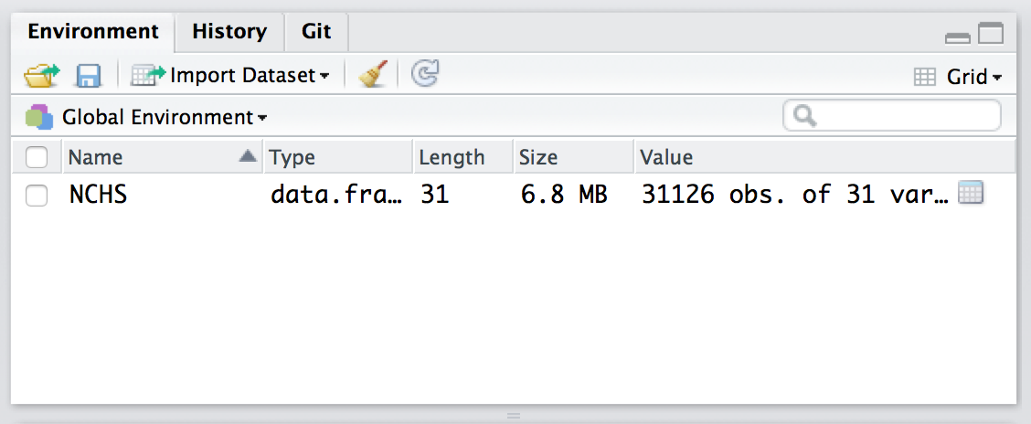
Figure 2.7: The session environment after the NCHS data table has been loaded.
If you haven’t already done so, go back to the beginning and type each command into the R console. Then find the environment tab and press the spreadsheet icon ![]() and the summary icon
and the summary icon ![]() .
.
You can look at the data table more closely by clicking on the small spreadsheet icon, ![]() . Finally, for data tables contained in a package, you can display a narrative description — the codebook — using the
. Finally, for data tables contained in a package, you can display a narrative description — the codebook — using the help() command:
2.7 Functions, arguments, and commands
The examples above demonstrate many of the most important components needed to use R. Giving these components names will help in communicating about using R.
Functions are the mechanism that R uses to carry out an operation. Functions transform one or more inputs into an output. You’ve seen several functions already: sqrt(), library(), data(), and help(). Functions have names. In this text, function names will be written followed by open and close parentheses simply to signal to you, the human reader, that the name refers to a function, as opposed to, say, NCHS, which is a data table, not a function.
Think of a function as a verb. It tells what to do.
A command is a complete statement of a computation. Commands are usually constructed by giving inputs to a function. Think of a command as a sentence.
The grammar of R sentences is straightforward. Follow the name of the function with a pair of parentheses. Inside the parentheses, you specify the input on which the operation is to be performed.
All of the commands shown here have this form: a function name followed by parentheses containing an argument.
sqrt(2)
library("dcData")
library("mosaicData")
data(package="dcData")
data(package="mosaicData")
data("NCHS")
help("NCHS")
You can also use an object name itself as a command.
This is useful when you want to get a quick display of the value stored under that name.2 Behind the scenes: Using an object name as a command is just shorthand for a command using the print() function. The explicit command would be print(NCHS) in this example."
The inputs to functions are called arguments. It would be reasonable to call the inputs to functions simply “inputs,” but that’s not the convention. Here are some of the arguments in the above examples:
The third example, package = "dcData" is called a named argument. Named arguments are a way to signal clearly what role the argument is to play. In the command data(package = "dcData") the name of the argument is package and the value "dcData" is the value given to that argument.
When there is more than one argument to a function, put them all in the same set of parentheses with a comma between the different arguments. For example, two arguments are specified here:
2.8 Objects
An object is a packet of information. The word “object” is not any more descriptive than, say, “thing”… at least “object” makes it clear that you are referring to a thing in R. Just about everything you’ll be using in R is an object. There are many different sorts of objects, just like there are many sorts of things in the world.
It helps to distinguish between the packet and the information contained in it. The information contained in the object is called its value. Most of the objects you will use have names, e.g. NCHS or sqrt. Sometimes you will use objects that don’t have a name, for instance the number 2 or the quoted set of characters "mosaicData". Here are some of the objects and their values that appear in the examples above:
| Name | Value | Kind of object |
|---|---|---|
NCHS |
data | a data table |
sqrt |
computer commands | a function |
"mosaicData" |
a string of characters | |
| 2 | a number | |
"NCHS" |
a string of characters |
It will take a while for you to get used to the difference between an object and the name of an object. Object names should never be in quotes and they should never begin with a digit. When quotes are used, it is to identify characters as a string. Strings are used for labels, or to identify something outside of R such as a web location, file name, or caption on a graphic.
Giving Names to Objects
Analyzing or visualizing data often involves several steps, each of which creates a new objects. It’s often useful to name these objects so that you can refer to them in the following steps.
Name an object with the <- notation. The syntax is simple:
In the jargon of computer programming, giving a name to an object is called assignment. You assign a name to an object.
Random sampling. It’s often useful to take a random subset of the cases in a data table.3 For instance, you might want to prototype with a small data table when developing your data wrangling and visualization before tackling the whole data table. The function that does this is called sample_n(). It takes two arguments: the name of the data table from which the subset is to be drawn and a named argument, size=, that specifies how many cases should be in the sample. For example:
By assigning the output of sample_n() to a named object, SmallNHCS in the statement above, you can access the object when you need it.
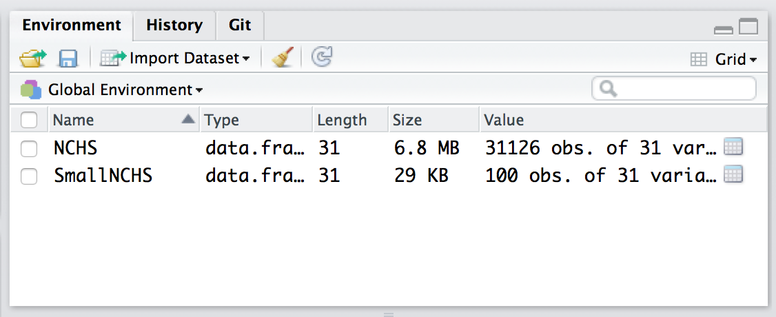
You can have as many named objects as you like. RStudio helps you keep track of them by listing them in the Environment tab, as in Figure 2.8.
Figure 2.8: When the SmallNCHS object is created, it appears in the Environment tab.
There are a few simple rules that apply when creating a name for an object:
The strikethrough bar, like ~this~, is not part of the name. The strikethrough is just a device in the notes to remind you that the name is not allowed.
- The name cannot start with a digit. So ~
100NCHSNCHS100is fine. This rule is to makes it easy for R to distinguish between object names and numbers. It also helps you avoid mistakes such as writing2piwhen you mean2*pi. - The name cannot contain any punctuation symbols (with two exceptions). So ~
?NCHSN*Hanes.and_in a name. - The case of the letters in the name matters. So
NCHS,nchs,Nchs, andnChs, etc. are all different names that only look similar to a human reader, not to R.
Occasionally, you will encounter function names like readr::read_csv(). This use of :: refers to a function contained in a specific package. In this case, the name refers to the read_csv() function in the readr package.
Example: Reading a file. The following command consists of a function whose argument is a quoted character string , that is, a sequence of characters taken literally as a value. Character strings always start and end with quotes, for instance, "My name is ..." or "Call me Ishmael". In contrast, quotes are not used with object names.
To read commands effectively, get in the habit of noticing strings and distinguishing them from object names. For instance, the following command contains a string, the assignment operator, and an object name.
The effect of this command is to read some data about internal combustion motors from a web site into an R object called Motors. Note that the URL of the data file is a quoted character string, but the function and object names are not quoted.
2.9 Exercises
Problem 2.1: The following ideas should be meaningful to you from the readings:
package, function, command, argument,
assignment, object, object name, data table,
named argument, quoted character string, value
Construct a working example R command that makes use of at least four of the ideas. Label which part of your example R command corresponds to each of those ideas.
Problem 2.2: Which of these kinds of names should be wrapped with quotation marks when used in R?
- function name
- file name
- the name of an argument in a named argument
- object name
Problem 2.3: Look at the documentation for the CPS85 data table in the mosaicData package. From reading that documentation, what is the meaning of CPS?
Problem 2.4: Consider these four relatively similar help( ) statements attempting to open the documentation page associated with CountryData found in the dcData package.
help(CountryData, package <- "dcData")help(CountryData, package = "dcData")help(package <- "dcData", CountryData)help(package = "dcData", CountryData)
Execute each of the four help( ) statements, one at a time, to answer the following questions. You may also find it useful to look at the documentation page for the help function itself by executing the following command in the console: ?help
Which one of the four
help( )statements is written to be most consistent with the recommendations in the chapter?Which one of the four
help( )statements does NOT work (i.e., produces an error message)?Challenge: Study the two remaining
help( )statements and the documentation for thehelpfunction itself. Explain how R can still execute them properly, even though they have been poorly specified. Hint: to assist your investigation, try replacing the word “package” with an unrelated word, like “bungalow” and see what happens.
Problem 2.5: Look at the help documentation for the library() function.
Without worrying about all the detail, answer these questions simply:
- What is the name of another function listed under “Usage” which has similar arguments to
library()? - In the “See Also” section of the documentation, what is the name of the function after
detach()?
Problem 2.6: Some of these are legitimate object names, others are not. For the ones that are not legitimate, say what is wrong.
essay14
first-essay
"MyData"
third_essay
small sample
functionList
FuNcTiOnLiSt
.MyData.
sqrt()
Problem 2.7: Install the nycflights13 package into R. (You can use the “Packages” tab which has an “install” button. If you are not using RStudio, given the R command install.packages("nycflights13"))
Once the package is installed, you can access the flights data table with this command:
The codebook is available with
Using the codebook and examining the data table with the View() command (hint: you’ll need to give flights as an argument to View()), answer these questions:
- How many variables are there?
- How many cases are there?
- What is the meaning of a case? (“Meaning” refers to the kind of entity, for instance, “airport” or “airline” or “date”. Hint: the case in
flightsis not any of these things.) - For each variable, is the variable quantitative or categorical?
- For the variables
air_timeanddistance, what are the units?
Problem 2.8: Consider this list of some possible mistakes in an assignment operation:
- No assignment operator
- Unmatched quotes in character string
- Improper syntax for function argument
- Invalid object name
- No mistake
For each of the following assignment statements, say what is the mistake.
ralph <- sqrt 10ralph2 <-- "Hello to you!"3ralph <- "Hello to you!"ralph4 <- "Hello to you!ralph5 <- date()
Problem 2.9: Here are a few characters:
. , ; _ - ^ [space] ( )
Which of those characters can be used in the name of an R object?
Which of those characters can be used in a quoted character string?
Problem 2.10: These questions should be easy to answer if you use the appropriate commands to load, view, or get documentation on the datasets.
- How many variables are there in
CountryData?
- What does the variable
tfatmeasure in theNCHSdata table? (in packagedcData) - How many cases are there in
WorldCities? - What’s the third variable in
BabyNames? - What are the codes for the levels of the categorical variable
partyin theRegisteredVotersdata table, and what does each code stand for?