Chapter 11 Modeling Randomness

The race is not to the swift, nor the battle to the strong, neither yet bread to the wise, nor yet riches to men of understanding, nor yet favor to men of skill; but time and chance happeneth to them all. – Ecclesiastes

Until now, emphasis has been on the deterministic description of variation: how explanatory variables can account for the variation in the response. Little attention has been paid to the residual other than to minimize it in the fitting process.

It’s time now to take the residual more seriously. It has its own story to tell. By listening carefully, the modeler gains insight into even the deterministic part of the model. Keep in mind the definition of statistics offered in Chapter 1:

Statistics is the explanation of variability in the context of what remains unexplained.

The next two chapters develop concepts and techniques for dealing with “what remains unexplained.” In later chapters these concepts will be used when interpreting the deterministic part of models.

11.1 Describing Pure Randomness

Consider an event whose outcome is completely random, for instance, the flip of a coin. How to describe such an event? Even though the outcome is random, there is still structure to it. With a coin, for instance, the outcome must be “heads” or “tails” – it can’t be “rain.” So, at least part of the description should say what are the possible outcomes: H or T for a coin flip. This is called the outcome set. (The outcome set is conventionally called the sample space of the event. This terminology can be confusing since it has little to do with the sort of sampling encountered in the collection of data nor with the sorts of spaces that vectors live in.)

For a coin flip, one imagines that the two outcomes are equally likely. This is usually specified as a probability, a number between zero and one. Zero means “impossible.” One means “certain.”

A probability model assigns a probability to each member of the outcome set. For a coin flip, the accepted probability model is 0.5 for H and 0.5 for T – each outcome is equally likely.

What makes a coin flip purely random is not that the probability model assigns equal probabilities to each outcome. If coins worked differently, an appropriate probability model might be 0.6 for H and 0.4 for T. The reason the flip is purely random is that the probability model contains all the information; there are no explanatory variables that account for the outcomes in any way.

Example: Rolling a Die

The outcome set is the possibilities 1, 2, 3, 4, 5, and 6. The accepted probability model is to assign probability 1/6 to each of the outcomes. They are all equally likely.

Now suppose that the die is “loaded.” This is done by drilling into the dots to place weights in them. In such a situation, the heavier sides are more likely to face down. Since 6 is the heaviest side, the most likely outcome would be a 1. (Opposite sides of a die are arranged to add to seven, so 1 is opposite 6, 2 opposite 5, and 3 opposite 4.) Similarly, 5 is considerably heavier than 2, so a 2 is more likely than a 5. An appropriate probability model is this:

Outcome	1	2	3	4	5	6
Probability	0.28	0.22	0.18	0.16	0.10	0.06

One view of probabilities is that they describe how often outcomes occur. For example, if you conduct 100 trials of a coin flip, you should expect to get something like 50 heads. According to the frequentist view of probability, you should base a probability model of a coin on the relative proportion of times that heads or tails comes up in a very large number of trials.

Another view of probabilities is that they encode the modeler’s assumptions and beliefs. This view gives everyone a license to talk about things in terms of probabilities, even those things for which there is only one possible trial, for instance current events in the world. To a subjectivist , it can be meaningful to think about current international events and conclude, “there’s a one-quarter chance that this dispute will turn into a war.” Or, “the probability that there will be an economic recession next year is only 5 percent.”

Example: The Chance of Rain

Tomorrow’s weather forecast calls for a 10% chance of rain. Even though this forecast doesn’t tell you what the outcome will be, it’s useful; it contains information. For instance, you might use the forecast in making a decision not to cancel your picnic plans.

But what sort of probability is this 10%? The frequentist interpretation is that it refers to seeing how many days it rains out of a large number of trials of identical days. Can you create identical days? There’s only one trial – and that’s tomorrow. The subjectivist interpretation is that 10% is the forecaster’s way of giving you some information, based on his or her expertise, the data available, etc.

Saying that a probability is subjective does not mean that anything goes. Some probability models of an event are better than others. There is a reason why you look to the weather forecast on the news rather than gazing at your tea leaves. There are in fact rules for doing calculations with probabilities: a “probability calculus.” Subjective probabilities are useful for encoding beliefs, but the probability calculus should be used to work through the consequences of these beliefs. The Bayesian philosophy of probability emphasizes the methods of probability calculus that are useful for exploring the consequences of beliefs.

Example: Flipping two coins.

You flip two coins and count how many heads you get. The outcome space is 0 heads, 1 head, and 2 heads. What should the probability model be? Here are two possible models:

If you are unfamiliar with probability calculations, you might decide to adopt Model 1. However heartfelt your opinion, though, Model 1 is not as good as Model 2. Why? Given the assumptions that a head and a tail are equally likely outcomes of a single coin flip, and that there is no connection between successive coin flips – that they are independent of each other – the probability calculus leads to the 1/4, 1/2, 1/4 probability model.

How can you assess whether a probability model is a good one, or which of two probability models are better? One way is to compare observations to the predictions made by the model. To illustrate, suppose you actually perform 100 trials of the coin flips in example above and you record your observations. Each of the models also gives a prediction of the expected number of outcomes of each type:

The discrepancy between the model predictions and the observed counts tells something about how good the model is. A strict analogy to linear modeling would suggest looking at the residual: the difference between the model values and the observed values. For example, you might look at the familiar sum of squares of the residuals. For Model 2 this is (28-25)² + (45-50)² + (27-25)². More than 100-years ago, it was worked out that for probability models this is not the most informative way to calculate the size of the residuals. It’s better to adjust each of the terms by the model value, that is, to calculate (28-25)²/25 + (45-50)²/50 + (27-25)²/25. The details of the measure are not important right now, just that there is a way to quantify how well a probability model matches the observations.

11.2 Settings for Probability Models

A statistical model describes one or more variables and their relationships. In contrast, a probability model describes the outcomes of a random event, sometimes called a random variable. The setting of a random variable refers to how the event is configured. Some examples of settings:

The number of radio-active particles given off by a substance in a minute.
A particular student’s score on a standardized test consisting of 100 questions.
The number of blood cells observed in a small area of a microscope slide.
The number of people from a random sample of 1000 voters who support the incumbent candidate.

In constructing a probability model, the modeler picks a form for the model that is appropriate for the setting. By using expert knowledge (e.g., how radioactivity works) and the probability calculus, probability models can be derived for each of these settings.

It turns out that there is a reasonably small set of standard probability models that apply to a wide range of settings. You don’t always need to derive probability models, you can use the ones that have already been derived. This simplifies things dramatically, since you can accomplish a lot merely by learning which of the models to apply in any given setting.

Each of the models has one or more parameters that can be used to adjust the models to the particular details of a setting. In this sense, the parameters are akin to the model coefficients that are set when fitting models to data.

11.3 Models of Counts

The Binomial Model

Setting. The standard example of a binomial model is a series of coin flips. A coin is flipped n times and the outcome of the event is a count: how many heads. The outcome space is the set of counts 0, 1, …, n.

To put this in more general terms, the setting for the binomial model is an event that consists of n trials. Each of those trials is itself a purely random event where the outcome set has two possible values. For a coin flip, these would be heads or tails. For a medical diagnosis, the outcomes might be “cancer” or “not cancer.” For a political poll, the outcomes might be “support” or “don’t support.” All of the individual trials are identical and independent of the others.

The name binomial – “bi” as in two, “nom” as in name – reflects these two possible outcomes. Generically, they can be called “success” and “failure.” The outcome of the overall event is a count of the number of successes out of the n trials.

Parameters. The binomial model has two parameters: the number of trials n and the probability p of success in each trial.

Example: Multiple Coin Flips

Flip 10 coins and count the number of heads. The number of trials is 10 and the probability of “success” is 0.5. Here is the probability model:

Outcome	0	1	2	3	4	5
Probability	0.001	0.010	0.044	0.117	0.205	0.246

Outcome		6	7	8	9	10
Probability		0.205	0.117	0.044	0.01	0.001

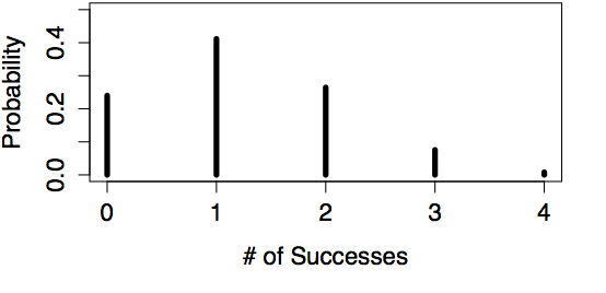
Examples of Binomial Models

n=4, p=0.30	n=100, p=0.30

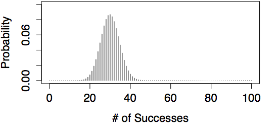Example: Houses for Sale

Count the number of houses on your street with a for-sale sign. Here n is the number of houses on your street. p is the probability that any randomly selected house is for sale. Unlike a coin flip, you likely don’t know p from first principles. Still, the count is appropriately modeled by the binomial model. But until you know p, or assume a value for it, you can’t calculate the probabilities.

The Poisson Model

Setting. Like the binomial, the Poisson model also involves a count. It applies when the things you are counting happen at a typical rate. For example, suppose you are counting cars on a busy street on which the city government claims the typical traffic level is 1000 cars per hour. You count cars for 15 minutes to check whether the city’s claimed rate is right. According to the rate, you expect to see 250 cars in the 15 minutes. But the actual number that pass by is random and will likely be somewhat different from 250. The Poisson model assigns a probability to each possible count.

Parameters. The Poisson model has only one parameter: the average rate at which the events occur.

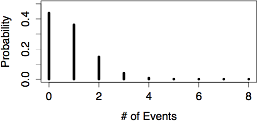
Example: The Rate of Highway Accidents

In your state last year there were 300 fatal highway accidents: a rate of 300 per year. If this rate continued, how many accidents will there be today?

Since you are interested in a period of one day, divide the annual rate by 365 to give a rate of 300/365 = 0.8219 accidents per day. According to the Poisson model, the probabilities are:

Outcome	0	1	2	3	4	5
Probability	0.440	0.361	0.148	0.041	0.008	0.001

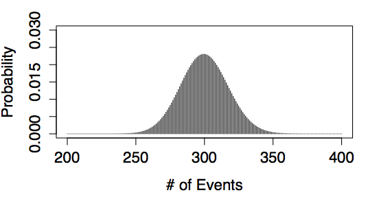
People often confuse the binomial setting with the Poisson setting. Notice that in a Poisson setting, there is not a fixed number of trials, just a typical rate at which events occur. The count of events has no firm upper limit. In contrast, in a binomial setting, the count can never be higher than the number of trials, n.

Examples of Poisson Models

rate = 0.8219	rate = 300

11.4 Common Probability Calculations

A probability model assigns a probability to each member of the outcome set. Usually, though, you are not interested in these probabilities directly. Instead, you want other information that is based on the probabilities:

Percentiles. Students who take standardized tests know that the test score can be converted to a percentile: the fraction of test takers who got that score or less. Similarly, each possible outcome of a random variable falls at a certain percentile. It often makes sense to refer to the outcomes by their percentiles rather than the value itself. For example, the 90th percentile is the value of the outcome such that 90 percent of the time a random outcome will be at that value or smaller.

Percentiles are used, for instance, in finding what range of outcomes is likely, as in calculating a coverage interval for the outcome.

Example: A Political Poll

You conduct 500 interviews with likely voters about their support for the incumbent candidate. You believe that 55% of voters support the incumbent. What is the likely range in the results of your survey?

This is a binomial setting, with parameters n = 500 and p = 0.55. It’s reasonable to interpret “likely range” to be a 95% coverage interval. The boundaries of this interval are the 2.5- and 97.5-percentiles, or, 253 and 297 respectively.

Quantiles or Inverse percentiles. Here, instead of asking what is the outcome at a given percentile, you invert the question and ask what is the percentile at a given outcome. This sort of question is often asked to calculate the probability that an outcome exceeds some limit.

Example: A Normal Year?

Last year there were 300 highway accidents in your state. This year saw an increase to 321. Is this a likely outcome if the underlying rate hadn’t changed from 300?

This is a Poisson setting, with the rate parameter at 300 per year. According to the Poisson model, the probability of seeing 321 or more is 0.119: not so small.

Calculation of percentiles and inverse percentiles is almost always done with software. The “computational technique” section gives specific instructions for doing this.

11.5 Models of Continuous Outcomes

The binomial and Poisson models apply to settings where the outcome is a count. There are other settings where the outcome is a number that is not necessarily a counting number.

The Uniform Model

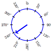
Setting. A random number is generated that is equally likely to be anywhere in some range. An example is a spinner that is equally likely to come to rest at any orientation between 0 and 360 degrees.

Parameters. Two parameters: the upper and the lower end of the range.

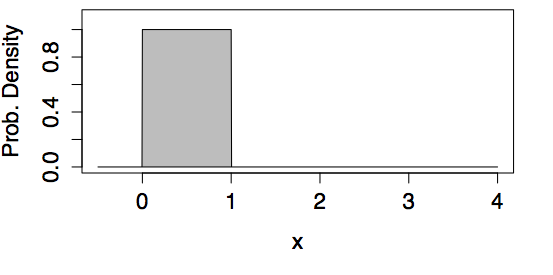
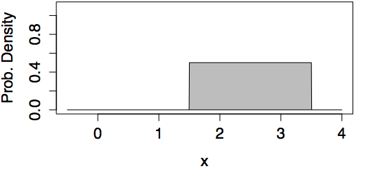
Examples of Uniform Models

min=0, max=1	min=1.5, max=3.5

Example: Equally Likely

A uniform random number is generated in the range 0 to 1. What is the probability that it will be smaller than 0.05? Answer: 0.05. (Simple as it seems, this particular example will be relevant in studying p-values in a later chapter.)

The Normal Model

Setting. The normal model turns out to be a good approximation for many purposes, thus the name “normal.” When the outcome is the result of adding up lots of independent numbers, the normal model often applies well. In statistical modeling, model coefficients are calculated with dot products, involving lots of addition. Thus, model coefficients are often well described by a normal model.

The normal model is so important that Section 11.5 is devoted to it exclusively.

Parameters. Two. The mean which describes the most likely outcome, and the standard deviation which describes the typical spread around the mean.

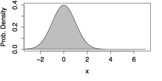
Examples of Normal Models

mean=0, std. dev.=1	mean=1.5, std. dev.=2

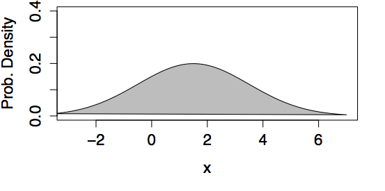Example: IQ Test Scores

Scores on a standardized IQ test are arranged to have a mean of 100 points and a standard deviation of 15 points. What’s a typical score from such a test? Answer: According to the normal model, the 95% coverage interval is 70.6 to 129.4 points.

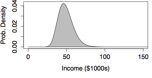
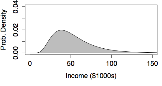
The Log-normal Model

Setting. The normal distribution is widely used as a general approximation in a large number of settings. However, the normal distribution is symmetrical and fails to give a good approximation when a distribution is strongly skewed. The log-normal distribution is often used when the skew is important. Mathematically, the log-normal model is appropriate when taking the logarithm of the outcome would produce a bell-shaped distribution.

Parameters. In the normal distribution, the two parameters are the mean and standard deviation. Similarly, in the log-normal distribution, the two parameters are the mean and standard deviation of the log of the values.

Example: High Income

In most societies, incomes have a skew distribution; very high incomes are more common than you might expect. In the United States, for instance, data on middle-income families in 2005 suggests a mean of about $50,000 per year and a standard deviation of about $20,000 per year (taking “middle-income” to mean the central 90% of families). If incomes were distributed in a bell-shaped, normal manner, this would imply that the 99th percentile of income would be $100,000 per year. But this understates matters. Rather than being normal, the distribution of incomes is better approximated with a log-normal distribution.(Montroll and Schlesinger 1983) Using a log-normal distribution with parameters set to match the observations for middle-income families gives a 99th percentile of $143,000.

Examples of Log-normal Models


logmean = 3.89, logsd=0.20	logmean = 3.89, logsd=0.47

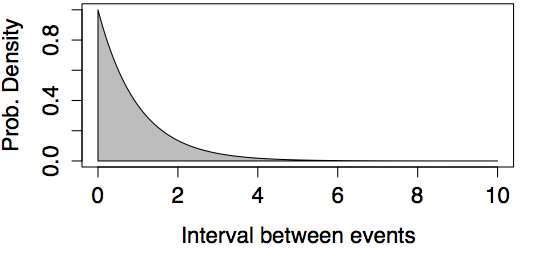
The Exponential Model

Setting. The exponential model is closely related to the Poisson. Both models describing a setting where events are happening at random but at a certain rate. The Poisson describes how many events happen in a given period. In contrast, the exponential model describes the spacing between events.

Parameters. Just like the Poisson, the exponential model has one parameter, the rate.

Example: Times between Earthquakes

In the last 202 years, there have been six large earthquakes in the Himalaya mountains. The last one was in 2005. [See update below.] This suggests a typical rate of 6 / 202 = 0.03 earthquakes per year – about one every 33 years. If earthquakes happen at random at this rate, what is the probability that there will be another large earthquake within 10 years of the last, that is, by 2015? According to the exponential model, this is 0.259. That’s a surprisingly large probability if you expected that earthquakes won’t happen again until a suitable interval passes. [Update: Tragically, there was another large earthquake in 2015. Events with a probability of 26% do happen.] There can also be surprisingly large gaps between earthquakes. For instance, the probability that another large earthquake won’t occur until 2105 is 0.05 according to the exponential model.

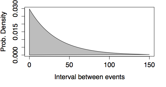
Examples of Exponential Models


Rate = 1	Rate = 0.03 (like the Himalayan earthquakes)

The Normal Distribution

Many quantities have a bell-shaped distribution so the normal model makes a good approximation in many settings. The parameters of the normal model are the mean and standard deviation. It is important to realize that a mean and standard deviation can be calculated for other models as well.

To see this, imagine a large number of trials generated according to a probability model. For the models discussed in this chapter, the outcomes are always numbers. So it makes sense to take the mean or the standard deviation of the trial outcomes.

When applied to probability models, the mean describes the center or typical value of the random outcome, just as the mean of a variable describes the center of the distribution of that variable. The standard deviation describes how the outcomes are spread around the center.

The calculation of percentiles, coverage intervals, and inverse percentiles is so common, that a shorthand way of doing it has been developed for normal models. At the heart of this method is the z-score.

The z-score is a way of referring a particular value of interest to a probability model or a distribution of values. The z-score measures how far a value is from the center of the distribution. The units of the measurement are in terms of the standard deviation of the distribution. That is, if the value is x in a distribution with mean $m$ and standard deviation s, the z-score is: z = (x - m) / s.

Example: IQ Percentiles from Scores.

In a standard IQ test, scores are arranged to have a mean of 100 and a standard deviation of 15. A person gets an 80 on the exam. What is their z-score? Answer: z = (80−100) / 15 = −1.33.

In some calculations, you know the z-score and need to figure out the corresponding value. This can be done by solving the z-score equation for x, or

x = m + s z.

Example: IQ Scores from Percentiles.

In the IQ test, what is the value that has a z-score of 2? Answer: x = 100 + 15×2 = 130.

Here are the rules for calculating percentiles and inverse percentiles from a normal model:

95% Coverage Interval. This is the interval bounded by the two values with z = −2 and z = 2.
Percentiles. The percentile of a value is indicated by its z-score as in the following table.

z-score	−3	−2	−1	0	1	2	3
Percentile	0.1	2.3	15.9	50	84.1	97.7	99.9

Values with z-scores greater than 3 or smaller than −3 are very uncommon, at least according to the normal model.

Example: Bad Luck at Roulette?

You have been playing a roulette game all night, betting on red, your lucky color. Altogether you have played n = 100 games and you know the probability of a random roll coming up red is 16 / 34. You’ve won only 42 games – you’re losing serious money. Are you unlucky? Has Red abandoned you?

If you have a calculator, you can find out approximately how unlucky you are. The setting is binomial, with n = 100 trials and p = 16/34. The mean and standard deviation of a binomial random variable are n × p and $\sqrt{n p (1-p)}$ respectively; these formulas are ones that all skilled gamblers ought to know. The z-score of your performance is:

\[ z = \frac{42 - 100 \frac{16}{34}}% {\sqrt{100 \frac{16}{34} (1 - \frac{16}{34}) }} = \frac{42 - 47.06}{5} = -1\]

The score of z = −1 translates to the 16th percentile – your performance isn’t good, but it’s not too surprising either.

When you get back to your hotel room, you can use your computer to do the exact calculation based on the binomial model. The probability of winning 42 games or fewer is 0.181.